Results and validation
Anisotropic diffusion
To validate the implementation of the algorithms for translational and rotationional diffusion introduced in Propagation of translational and angular motion I use the same example as in [13]. Here, the translational and rotational diffusion tensors do not represent any specific molecule:
In order to validate the algorithm, the mean squared displacement (MSD) and rotational time correlation are compared with theory. The mean squared displacement (MSD) is given by
The rotational time correlation function is given by [92]:
where \(\hat{\boldsymbol{n}}_l(t)\) are the unitary vectors that describe the current orientation of the molecule at time point \(t\) for each of the 3 rotation axis (\(l \in {1,2,3}\)). Fig. 25 compares the simulation results to the theoretical prediction, which, for the rotational time correlation function, is given by a multi-exponential decay function [92]:
The relaxation times are given by
\(D^{rr,b}_1, D^{rr,b}_2, D^{rr,b}_3\) are the eigenvalues of the rotational diffusion tensor \(\boldsymbol{D}^{rr,b}\) in the molecule frame and D is the scalar rotational diffusion coefficient given by \(D = \frac{Tr(\boldsymbol{D}^{rr,b})}{3}\). Parameter \(\Delta\) is given by
The amplitudes of the individual exponential decays are given by
with \(F_l = - \frac{1}{3} + \sum_{k=1}^3 \hat{n}_{l,k}^4\) and \(G_l=\frac{1}{\Delta}\Big( -D + \sum_{k=1}^3 D^{rr,b}_k \Big[ \hat{n}_{l,k}^4 + 2 \hat{n}_{l,m}^2 \hat{n}_{l,n}^2 \Big] \Big)\), where \(m, n \in \{1,2,3\}-\{k\}\).
If we choose the normal vectors of each axis \(\hat{\boldsymbol{n}}_l\) such that these are identical with the basis vectors of the local frame, i.e. \(\hat{\boldsymbol{n}}_1 = \boldsymbol{e}_x = [1,0,0]\), \(\hat{\boldsymbol{n}}_2 = \boldsymbol{e}_y = [0,1,0]\), \(\hat{\boldsymbol{n}}_3 = \boldsymbol{e}_z = [0,0,1]\), \(a_2-a_3\) vanish such that we end up with a double exponential decay (Fig. 25 B).
Fig. 25 shows that the rotation and translation propagators result in the correct mean squared distribution and rotational time correlation.
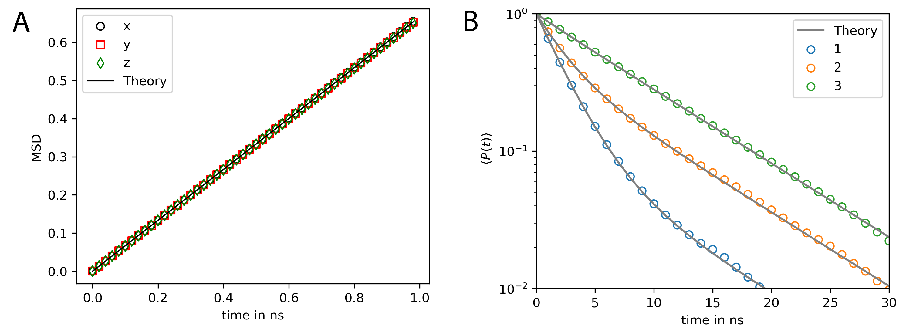
Fig. 25 MSD and rotational relaxation times of a rigid bead molecule matches the theoretical prediction. (A) Mean squared displacement (MSD) of the rigid bead molecule computed with PyRID. The displacement in each dimension (colored markers) is in very good agreement with the theory (black line). (B) The rotational relaxation of the rigid bead molecule is also in close agreement with the theory (gray lines, Eqs.(54)-(55)) for each of the the rotation axes (colored markers).
Diffusion tensor of igG3
The methods outlined in section Mobility tensor for rigid bead models have, at least to my knowledge, only been implemented in the freely available tool Hydro++. The source code for Hydro++ is, however, not publicly available. To efficiently set up a system of rigid bead molecules, the method has now also been implemented directly into PyRID. The implementation is tested against Hydro++ using a model of the protein igG3 that comes with the documentation of Hydro++. The results are in good agreement at up to 4 digits (Table 1.4). The slight difference is probably due to numerical errors that accumulate when numerically inverting the large supermatrices.
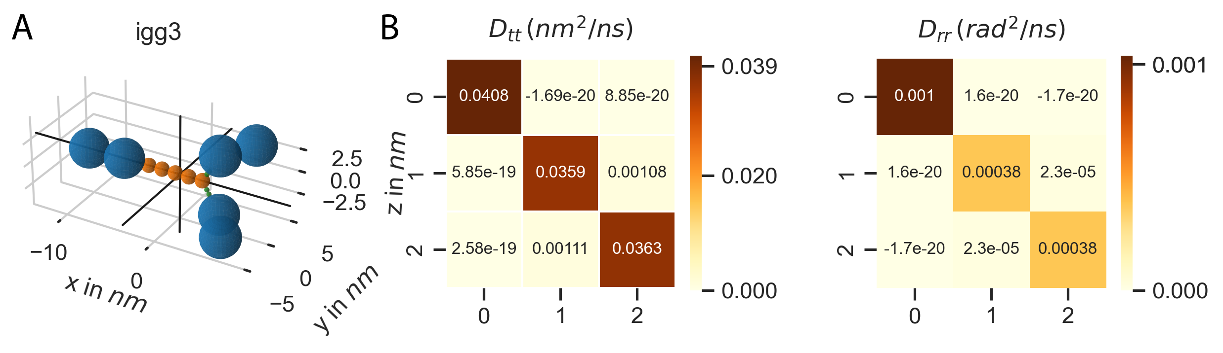
Fig. 26 The diffusion tensor of igG3 calculated with PyRID. (A) Rigid bead molecule representation of igG3 as found in de la Torre and Ortega [93]. The black cross marks the center of diffusion. (B) Translational and rotational diffusion tensor of igG3. A comparison of the result from PyRID with those of the Hydro++ suite can be found in table 1.4.

Fig. 27 Translational and rotational diffusion tensors of the IgG3 rigid bead model. Here, the result from PyRID is compared to the result gained from the Hydro++ suite. We find small deviations originating from numerical errors that build up mainly during the super-matrix inversion calculations.
Fixed concentration boundary
As mentioned in the methods chapter, fixed concentration boundary conditions couple the simulation box to a particle bath. Thereby, we can simulate, e.g., a sub-region within a larger system without the need to simulate the dynamics of the molecules outside simulation box directly. As an example system we take a 3d model of synapse. The post- and presynaptic spine are both contained inside the simulation volume whereas dendrite and axon are cutoff at the simulation box boundary (Fig. 28 A). We define three molecular species: Species A diffuses in the volume outside the spines (in the extracellular space), species B is located inside the postsynaptic spine and species C on the surface (within the membrane) of the postsynaptic spine. All species consist of a single particle with radius \(2\,nm\). The diffusion coefficient is calculated from the the Einstein relation where the temperature is set to \(293.15\,K\). The viscosity is set to \(1\,mPa\cdot s\) and the time step to \(10\,ns\). The simulation box size is set to \(250\,nm \cdot 250\,nm \cdot 350\,nm\). At the beginning there are no molecules inside the simulation box. However, the outside concentration of each species is set to \(1000\) molecules per total volume or total surface area respectively. Thereby, there should be 1000 molecules of each species in the volume and on the surface of each compartment as soon as the system has reached its equilibrium state. Indeed, after about \(0.5\,ms\) the system has reached equilibrium and the number of each species fluctuates around the number 1000 (Fig. 28 B). As one would expect, species A fills the simulation volume the fastest as the boundary area is the largest. Species B and C which are located in the volume and on the surfaces of the postsynaptic compartment fill the simulation volume at about the same rate.
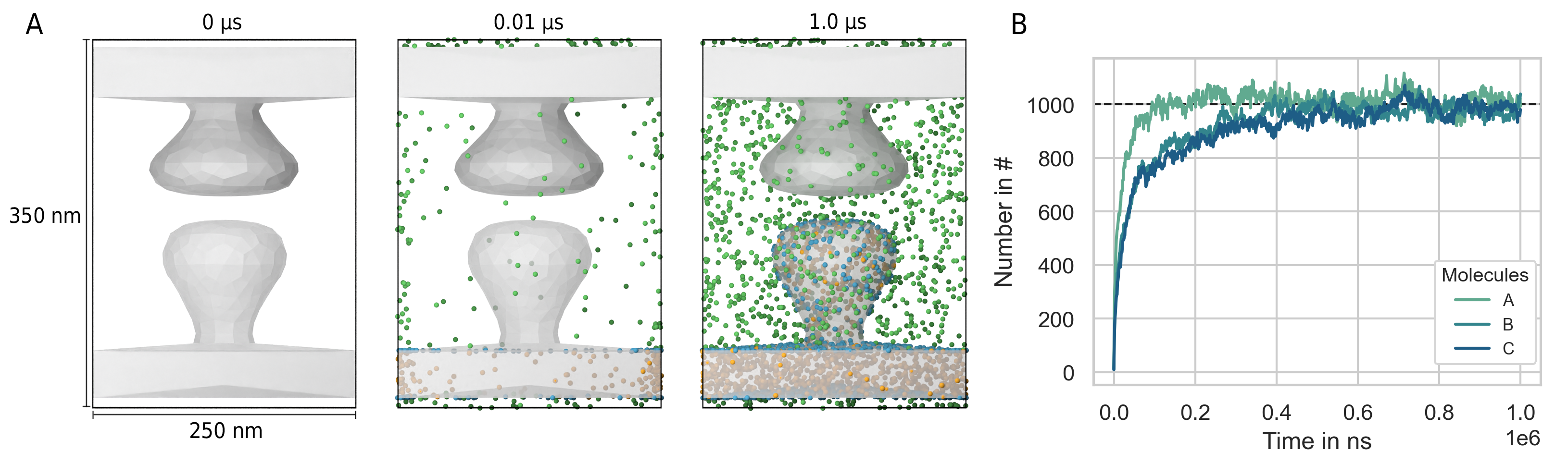
Fig. 28 Fixed concentration boundary conditions result in the system approaching a target molecule concentration per compartment. (A) We start with an empty scene (left). However, because the molecule concentration of virtual molecules outside the simulation box is above zero, surface and volume molecules enter the system via the boundary (middle). After around 500 ns, the molecule concentration inside the simulation box reaches the target concentration (A) right, (B).
Choosing the right reaction rate and radius
pyrid.reactions.reactions_util.k_macro
pyrid.reactions.reactions_util.k_micro
As described in [86], the reaction radius \(R_{react}\) may be interpreted as the distance at which two particles can no longer be treated as moving independently, because there interactions becomes significant. Furthermore, Schöneberg and Noé [86] suggest that the length scale of electrostatic interactions can be used to define \(R_{react}\). In general, the reaction radius should not be so large that in dense settings molecules would react with a partner that is not among the nearest neighbours. However, \(R_{react}\) should also not be smaller than the average change in the distance between molecules, which is given by \(\lambda_{AB} = \sqrt{4(D^t_A +D^t_B) \Delta t}\), where \(D^t_A\) and \(D^t_B\) are the translational diffusion constants of two molecular species \(A\) and \(B\). Otherwise, a molecule might pass many reaction partners in between two time steps where the bi-molecular reactions are not evaluated [94]. However, even if \(\lambda_{AB} \approx R_{react}\) the system would still correctly reproduce the deterministic rate equation description of the reaction kinetics. Of course, in any case, \(R_{react}\) should not be chosen smaller than the radius of excluded volume of the molecule species in the presence of repulsive interactions. A description of the reaction kinetics in terms of a system of differential equations assumes a well mixed system. Therefore, the simulation results are also only directly comparable with the ODE approach, if the reactions are reaction rate limited, not diffusion limited such that the system has enough time to equilibrate in between reactions. Let us take a very simple example where \(\ce{A + B -> C }\). If the reaction kinetics are diffusion limited, the reaction products do not have enough time to mix with the rest of the system. Thereby, regions of low educt concentration evolve where reactions had occurred, while in the regions where no reactions occurred yet, the concentration of educts stays approximately same as in the beginning. Therefore, for the remaining educts in the system, the probability of encounter stays approximately the same. In contrast, if we assume a well stirred system, the concentration of educts would globaly decrease in time, lowering the probability of educt encounters. Therefore, the reaction kinetics are sped up in the stochastic simulation compared to the ode approach (Fig. 29). Interestingly, Schöneberg and Noé [86] found exactly the opposite effect, as the reaction kinetics where slowed down in the stochastic simulation. The reason for this discrepancy in the results is unclear. However, I simulated the very same system in ReaDDy and got the same result as with PyRID.
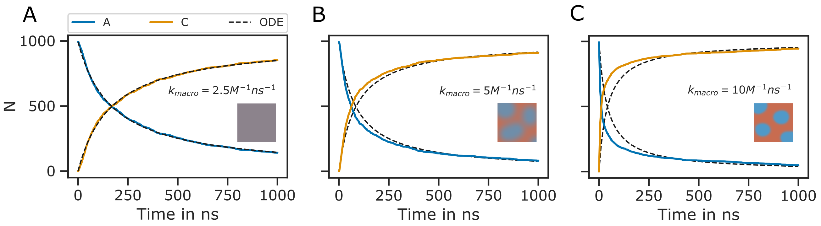
Fig. 29 Diffusion limited bi-molecular reactions are not accurately described by ODEs. Shown is the minimal system \(\ce{A + B ->[\ce{k_1}] C }\) with \(R_{react} = 4.5 nm\) and \(\sigma_A = 3 nm\), \(\sigma_B = 4.5 nm\), \(\sigma_C = 3.12 nm\). The same system has been used for validation of ReaDDy in [86]. The ODE approach to the description of the reaction kinetics assumes a well mixed system. If the reaction rate is small, the system has enough time to equilibrate in between reactions and the ODE approach (black dotted lines) and the particle-based SSA approach (colored lines) match (A). As the reaction rate increases (B-C) this is no longer the case, as the system is no longer well mixed at any point in time. Here, the system can be divided into regions of high and low educt concentrations (depicted by the small insets). Thereby, at the onset, the reaction kinetics in the stochastic simulation are faster than predicted by the ODE approach (B, C). However, when a critical mass of educts have reacted, the slow diffusion has an opposite effect on the reaction kinetics as the probability of isolated single educts to collide becomes lower than in the well mixed case. The slow down effect is especially prominent in B, C at around 500 ns. The reaction kinetics are therefore better described by two exponential functions instead of one.
Given a reaction radius \(R_{react}\), we would like to know at what microscopic reaction rate \(k\) a simulation would match an experimentally measured macroscopic reaction rate \(k^{macro}\). For two non-interacting molecule species \(A\) and \(B\) with translational diffusion constants \(D^t_A\) and \(D^t_B\) and \(\lambda_{AB}<<R_{react}\), \(k_{macro}\) is given by [94]
Equation (56) can solved numerically for \(k\). Also, if the \(k \rightarrow \infty\), (56) simplifies to the Smoluchowski equation where we can express the reaction radius in terms of the macroscopic reaction rate [94]:
In the limit where \(k << \frac{D_A^t+D_B^t}{R_{react}^2}\), Eq. (56) can be Taylor expanded and simplifies to [94]:
The above equations are, however, only valid in the case where molecules are represented by single particles and also only in 3 dimensions. PyRID has a build in method to calculate the reaction rates and radii based on equation (56).
Bi-molecular reactions between rigid bead molecules
The representation of molecules by single particles neglects the complex structure of molecules. Bi-molecular reactions between proteins can occur via different reaction sites. Therefore, also here, the isotropic picture breaks down. PyRID enables the simulation of reactions between complex molecules having different reaction sites. Different reaction sites are represented by beads/patches that are part of the rigid bead molecules topology. Similar to uni-molecular reactions, bi-molecular reactions can be defined on particles or molecules. However, because PyRID only computes the distances between the particles in the system, also reactions that are defined on the molecule level need to be linked to a particle type pair. If the the two particles are within the reaction distance and if the reaction is successful, the reaction itself will, however, be executed on the respective molecule types. As an example, we again consider the simple system \(\ce{A + B <=>[\ce{k_1}][\ce{k_{-1}}] C }\). However, molecules \(A\) and \(B\) are each represented by two beads \(a_1, a_2\) and \(b_1, b_2\). Also, we add another reaction path \(\ce{A + B ->[\ce{k_2}] D }\). We now may define reactions for different pair permutations of the available beads:
where \(k_i\) are the microscopic reaction rates and \(R_i\) the reaction radii. For better visualization, also see Fig. 30 A and B. As such, molecules \(A\) and \(B\) can undergo fusion to molecule \(C\) via three pathways, defined by three bead pairs \((a_1, b_1), (a_1, b_2), (a_2, b_2)\). Whereas for the particle pairs \((a_1, b_2)\) and \((a_2, b_2)\) only one reaction pathway is defined respectively, for the particle pair \((a_1, b_1)\) a second reaction path has been defined for the fusion of molecules \(A\) and \(B\) to molecule \(D\). We may also describe this system in terms of a system of ODEs:
The macroscopic rate constants \(k_{macro}^i\) can be calculated from Eq. (56). Note, however, that for more complex molecules Eq. (56) does not hold true, because we would also need to take into account the rotational motion of the molecule in addition to the translational diffusion constant that describes the motion of the molecule center. In our example, the bead motion is, however, close enough to that of a single spherical particle such that the results from the Brownian dynamics simulation are in close agreement with the ODE formulation (Fig. 30 C).
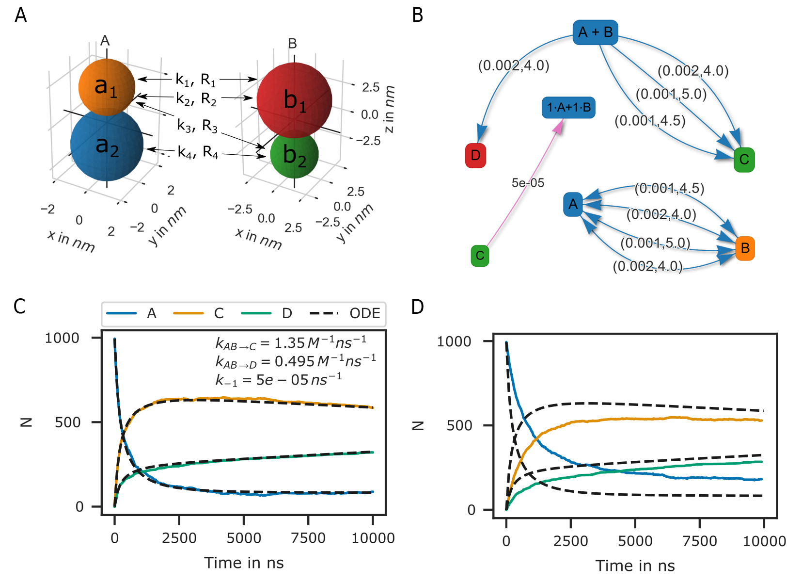
Fig. 30 Bi-molecular reaction between two rigid bead molecules.(A) Depiction of the two rigid bead molecules and the different reactions defined on their respective particles/beads. (B) Reaction graphs showing the different reaction paths for the fusion reactions \(\ce{A + B -> C}\) and \(\ce{A + B -> D}\) as well as the fission reaction \(\ce{C -> A + B}\). The lower right graph simply depicts the different reaction paths between the two educts A and B without specifying the products. In total there are 4 paths (Eq. (59)). (C) If not accounting for any repulsive interaction between molecules A and B, the simulation results are in good agreement with the ODE description (Eq. (60)). (D) However, if we account for the excluded volume of the molecules by a repulsive interaction potential, the results of the two approaches (particle dynamics and ODE description) differ.
At this point one might argue that there is only little to no benefit of the rigid bead model description over other SSA schemes. And in principle that is true. Systems such as the above could also be modeled using single particle Brownian dynamics or even ODEs. However, if we take into account the excluded volume of the molecules by introducing a repulsive interactions between the beads, the reaction kinetics differ from the ODE solution (Fig. 30 D). The bead radii are chosen equal to the reaction radius, where \(\sigma_{a_1} = 2.0 nm\), \(\sigma_{a_2} = 1.5 nm\), \(\sigma_{b_1} = 2.0 nm\), \(\sigma_{b_2} = 3.0 nm\). Thereby, the molecules react upon contact. For such simple molecules one could, however, neglect the bead topology and approximate the molecules by single beads with repulsive interactions and get a very similar result. For more complex molecules where the reaction volumes are much more anisotropic, one would, however, expect a larger deviation from the repulsive sphere approximation. The benefits of the rigid bead model approach become more important when we consider binding reactions.
Reactions between surface molecules
As a model, let us consider a four component system and implement a simple autocatalytic reaction scheme. The system consists of a freely diffusing transmembrane molecule \(U\). In addition, we add a second, freely diffusing, surface molecule \(P\). Let \(U\) and \(P\) form a complex \(B\) via a fusion reaction:
The reaction rates are set to \(k_{on} = 1e-5 ns^{-1}\) and \(R_{react}= 4nm\). In addition, we add an enzymatic/katalytic reaction:
We also account for a reverse reaction where
Here, \(k_{enz} = 1e-3 ns^{-1}\), \(k_{-enz} = 5e-5 ns^{-1}\) and \(R_{react}= 4nm\). The reaction product \(P^{\prime}\) has a much higher binding affinity for \(U\):
with \(k_{on}^{\prime} = 1e-2 ns^{-1}\) and \(R_{react}= 4nm\) (note that \(k_{on}^{\prime} >> k_{on}\)). The break up of the complex is accounted for by a fission reaction
As expected from an autocatalytic reaction, the product \(B\) follows a sigmoid function (Fig. 31). We may compare the simulation result to the corresponding ODE description. The above system expressed in terms of a system of ODEs reads
However, equation (56) is only valid in the 3D case and a solution for the 2D case is difficult to derive as the rate constant is concentration dependent. A closed form analytical expression has not yet been derived for the Doi scheme [94, 95, 96, 97]. A more in depth discussion on this topic and theoretical results for the Smoluchowski theory can be found in [98]. However, for the current system the simulation result can be matched using a constant reaction rate \(k_{macro}^{2D} = k_{macro}/5.6\) despite the decay in molecule density over time (Fig. 31 A). A closed form expression for \(k_{macro}\) is extremely useful when setting up a reaction diffusion simulation. Even if results do not match exactly, the ODE approach can help to choose the correct parameters for a particle-based simulation that might take several order longer than solving the system of ODEs. Whereas the ODE description is useful in many regards, we usually decide to do a particle based simulation because we are interested in settings that are not well mixed, or where interactions between molecules play a role.
Toy model of the PSD
As an example, where the particle-based approach becomes essential, we may transfer the autocatalytic system from above to a simplified model of the postsynapse. In our new setting, \(P\), \(P^{\prime}\) and \(B\) no longer diffuse but are fixed to a region that we interpret as being the PSD. In addition, a 3d mesh of a postsynaptic spine is introduced to the simulation and species \(U\) enters the simulation volume where the extrasynaptic region intersects the simulation box via a fixed concentration boundary. \(P\) now represents a receptor binding site, \(U\) the freely diffusing receptors and \(B\) the bound receptor or an occupied binding site. In this adapted system the autocatalytic reaction scheme results in receptor clustering (Fig. 31 B). Note that whereas the reaction \(\ce{B + P ->[\ce{k_{enz}}] B + P^{\prime} }\) is implemented as an enzymatic reaction in PyRID, the physical interpretation could be very different. For example, the conversion of \(\ce{P -> P^\prime}\) could occur only indirectly via the complex \(B\) and by a local signaling pathway that includes other molecules that we do not model here explicitly. Important is only that this pathway is triggered by \(B\) and that it is locally restricted for receptor clusters to evolve.
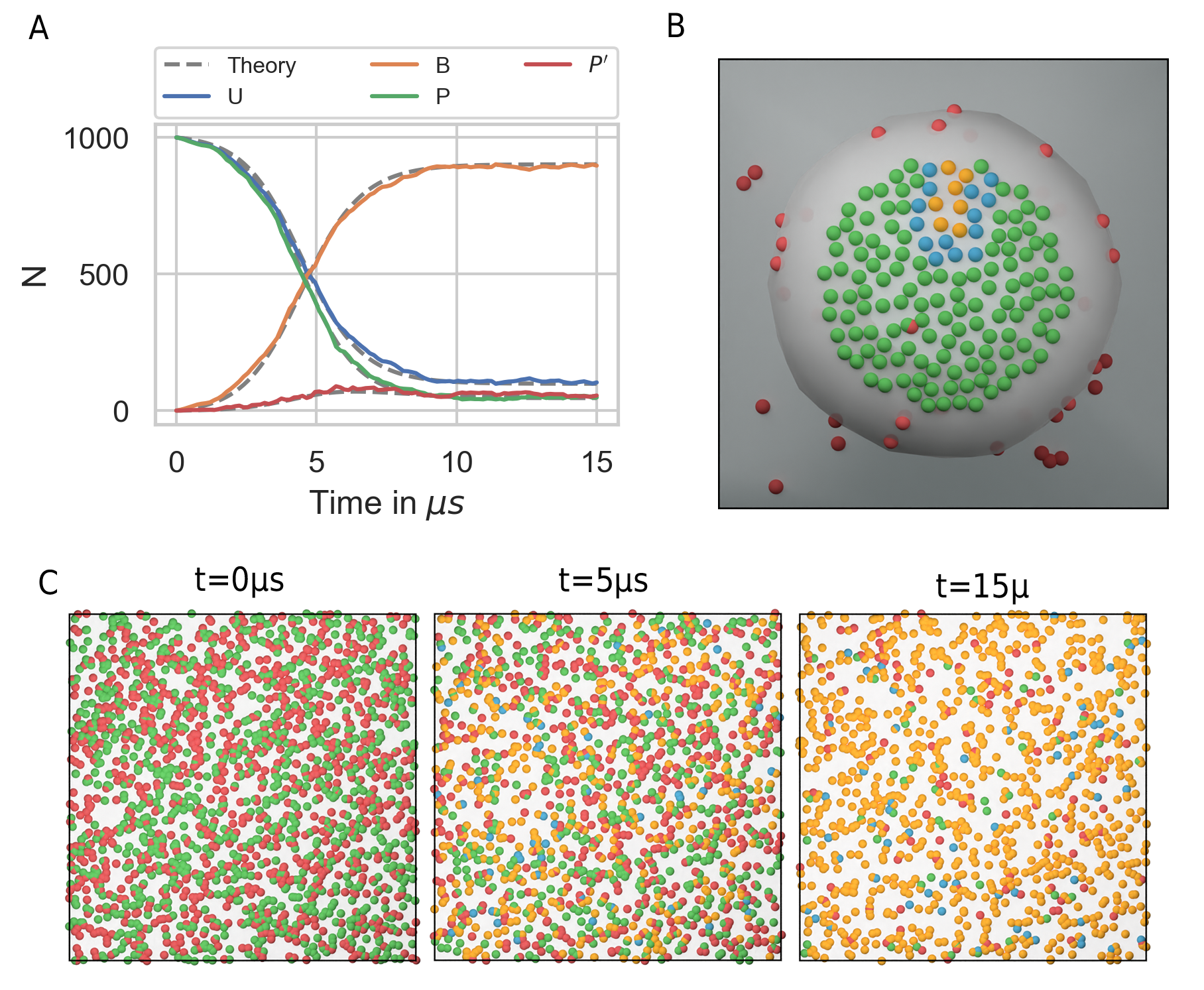
Fig. 31 Autocatalytic reaction diffusion system in 2D. (A) Number of the different molecular species evolving according to the reactions defined by equations (61)-(65). The simulation results are matched by the ODE description by fitting the macroscopic reaction rates (dotted grey lines). (B) Toy model of the PSD. Using the reaction scheme defined by equations (61)-(65) but fixing the position of species \(P\), \(P^{\prime}\) and \(B\) we observe the formation of species cluster (\(U\) in red, \(P\) in green, \(P^{\prime}\) in blue and \(B\) in yellow). (C) Evolution of the autocatalytic reaction system shown in (A) at different points in time (\(U\) in red, \(P\) in green, \(P^{\prime}\) in blue and \(B\) in yellow).
Hard sphere fluid
A hard sphere fluid is very useful for validation as there exist analytic expressions for the radial distribution function but also for the pressure.
Radial distribution function
Fig. 32 shows the radial distribution function for a hard sphere fluid that is modelled using the harmonic repulsive interaction potential (Eq. (51)). The sphere diameter is set to \(1\,nm\). The simulation result is is in good agreement with a closed-form analytical expressions of the hard sphere radial distribution function [99] (Fig. 32 B). The analytical expression for the radial distribution function is too long to be presented here. The interested reader is referred to [99].
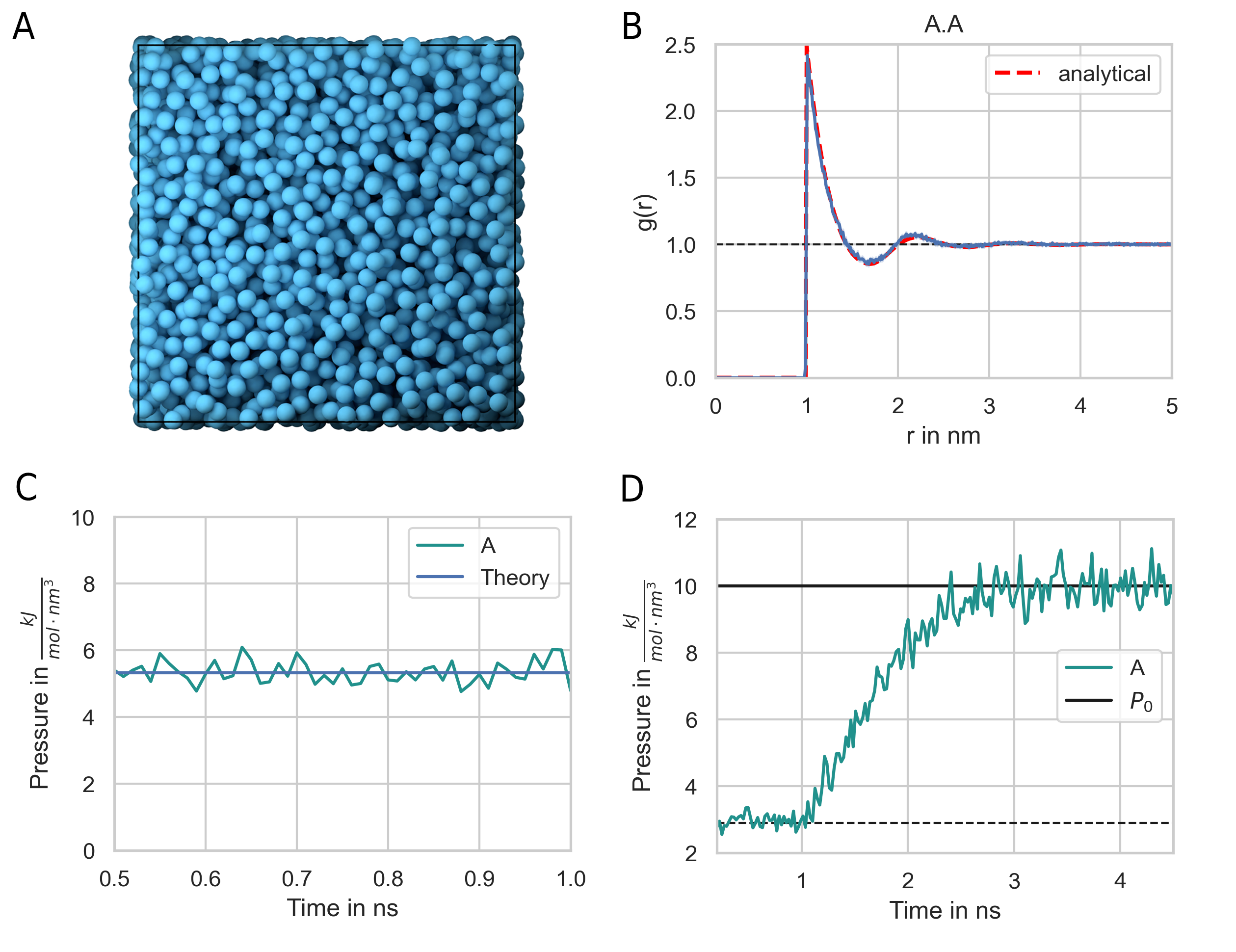
Fig. 32 Hard-sphere radial distribution function. (A) The system is set up with a packing fraction of \(\eta = 0.3\). The particle diameter is set to 1 nm and pair interactions occur via a harmonic repulsive potential. (B) The resulting radial distribution function (blue line) is in close agreement with theoretical prediction (red line). (C) The pressure of the hard-sphere fluid obtained from simulations is also in close agreement with theory [99]. (D) A hard-sphere fluid NPT ensemble simulation. From time 0.5 ns, the Berendsen barostat is activated and drives the system to the target pressure \(P_0 = 10\, \text{kJ}/(\text{mol}\, \text{nm}^3) = 16.6\, \text{MPa} = 166\, \text{bar}\) .
Pressure
We can use a hard sphere fluid for validation of the pressure calculation. For a hard sphere fluid, an analytical expression for the pressure is given in terms of the radial distribution function at contact and the second virial coefficient [100]:
where \(\sigma\) is the hard-sphere diameter, \(\rho\) the number density and \(b = (2 \pi/3) \sigma^3\) the second virial coefficient. The radial distribution function at contact can be approximated by the solution to the Percus-Yevick equation [101]:
where \(\eta = (\pi/6) \rho \sigma^3\) is the packing fraction. The pressure obtained from the simulation of a hard sphere fluid is in close agreement with this theoretical result (Fig. 32 C). In addition, the system does reach the target pressure using the Berendsen barostat (Fig. 32 D)
LLPs of Patchy Particles
Liquid-liquid phase separation (LLPS) gained a lot of interest in recent years as more experimental evidence has been gathered that many cell structures are formed by LLPS. LLPS is a compelling mechanism as it might answer, how cells are able to organize in the presence of a crowded environment with thousands of molecular species [61]. Examples include nucleoli, Cajal bodies, stress granules but also the PSD [58]. In an number of papers Zeng et al. have shown that many of the proteins found in the PSD are able to phase separate [58, 59, 60]. We would like to better understand the phase behaviour of the PSD as this might have an impact especially on the expression of late phase LTP. PSD substructures change in morphology within half an hour or stay rigid for many hours [62], indicating that the PSD might switch back and forth between crystalline, gel like and liquid states. Another study has shown that synaptic nanomodules, including the PSD are reallocated and change in size in response to synaptic plasticity induction [54, 57]. The issue that arises when investigating the phase behaviour of complex molecules is that even modern computers are able to only simulate 10-20 small proteins [90]. Therefore, coarse graining methods are needed. With models that describe the disordered region of proteins on the level of amino-sequences simulations with a few hundred copy numbers are already feasible [72, 90]. A minimal coarse graining approach represents proteins by patchy particles where the multivalent interaction sites of the proteins are modeled by attractive patches whereas the excluded volume is represented by a core particle with repulsive interactions. Espinosa et al. [90] have used such a model to investigate the stability and composition of biomolecular condensates. PyRID is well suited for simulations of patchy particles. For validation I here reproduce one of the results from Espinosa et al. [90]. In their work, patches interact via an attractive square well interaction potential [29]:
where \(\alpha = 0.01 \sigma\) with \(\sigma\) being the hard sphere radius. The core particles interact via a pseudo hard sphere potential [31]:
where \(\lambda_a = 49\) and \(\lambda_r = 50\). \(\epsilon_R\) is the energy constant, \(r_w\) is the radius of the attractive well and \(\alpha\) determines the steepness of the potential well edge. To ensure that each patch does at maximum interact with one other patch at any time, in [90] \(r_w\) has been set to \(0.12 \sigma\). Here, I did the same, however, note that thanks to the ability to define binding reactions in PyRID we could in principle also choose a larger radius for the attractive interaction potential. To compute the phase diagram/the coexistence curve for a patchy particle fluid, [90] used the direct coexistence method. The system is initialized at a volume density of \(\approx 0.3\) in a cubic box with \(2000\) patchy particles and at a temperature of \(179.71 K\). Periodic boundary conditions are used. The integration time step was set to \(2.5 ps\). A small integration time step is necessary due to the very short and steep attractive interaction between patches. Note that for Brownian dynamics simulations one would ideally use a weaker, soft interaction potential. Also, for such small integration time steps, the Brownian assumption is not necessarily valid anymore, e.i. the diffusive motion is not accurately described by a Markov process. However, we will see that, nevertheless, the results from [90] can be reproduced fairly accurately using the Brownian dynamics approach. In the following I briefly describe the direct coexistence method as used in [90]. In a first step, the patchy particle fluid is equilibrated in an NPT simulation at zero pressure and an energy constant \(\epsilon_{CSW}\) that is high enough to ensure phase separation. Thereby, the value of \(\epsilon_{CSW}\) depends on the system temperature and the patchy particle valency. As a rule of thumb, \(\frac{k_B T}{\epsilon_{CSW}}\) should be smaller than \(0.1\). For the equilibration phase I used the highest value that is given in table 1.5 for the different valencies respectively. After the equilibration phase the simulation box is elongated along the x-axis by a factor of 3. Thereby, a two phase system is created with infinite dense and dilute sheets. The elongated system is then simulated in the NVT ensemble for various different values of \(\epsilon_{CSW}\) (see table 1.5). The simulation is continued until the system reaches a new equilibrium, which was the case after \(\approx 2e7\) steps at approximately \(120\, it/s\). Thereby, a single simulation took \(\approx 2\, days\). In total 33 such simulations, 11 for each of the three valency cases, were executed on a high compute cluster. In a final step, a concentration profile is sampled, from which the volume fraction of the dense and dilute phase are estimated [30]. I found that the coexistence curves acquired with PyRID were in good agreement with [90] (Fig. 33). However, for the 5-valency case, Espinosa et al. [90] found a slightly higher volume fraction in the dense phase close to the critical point. Also, Espinosa et al. [90] found that the coexistence curve shows minimum below the critical for the 4-valence case, which I did not observe. The reason could lie in inaccuracies that are a result of to the Brownian approximation. More probable is, however, that the choice of the thermostat is responsible for the discrepancy as Espinosa et al. [90] used a Nosé-Hoover thermostat instead of a Langevin thermostat. However, I would argue that a Langevin thermostat, or in this case overdamped langevin dynamics/Brownian dynamics, represent the dilute phase more accurately as it accounts for the interaction with the solvent molecules.
valency |
\(\epsilon_{CSW}\) in \(\frac{kJ}{mol}\) |
|---|---|
sites |
\(14.5-23.3\) |
sites |
\(12.0-20.0\) |
sites |
\(10.5-16.0\) |
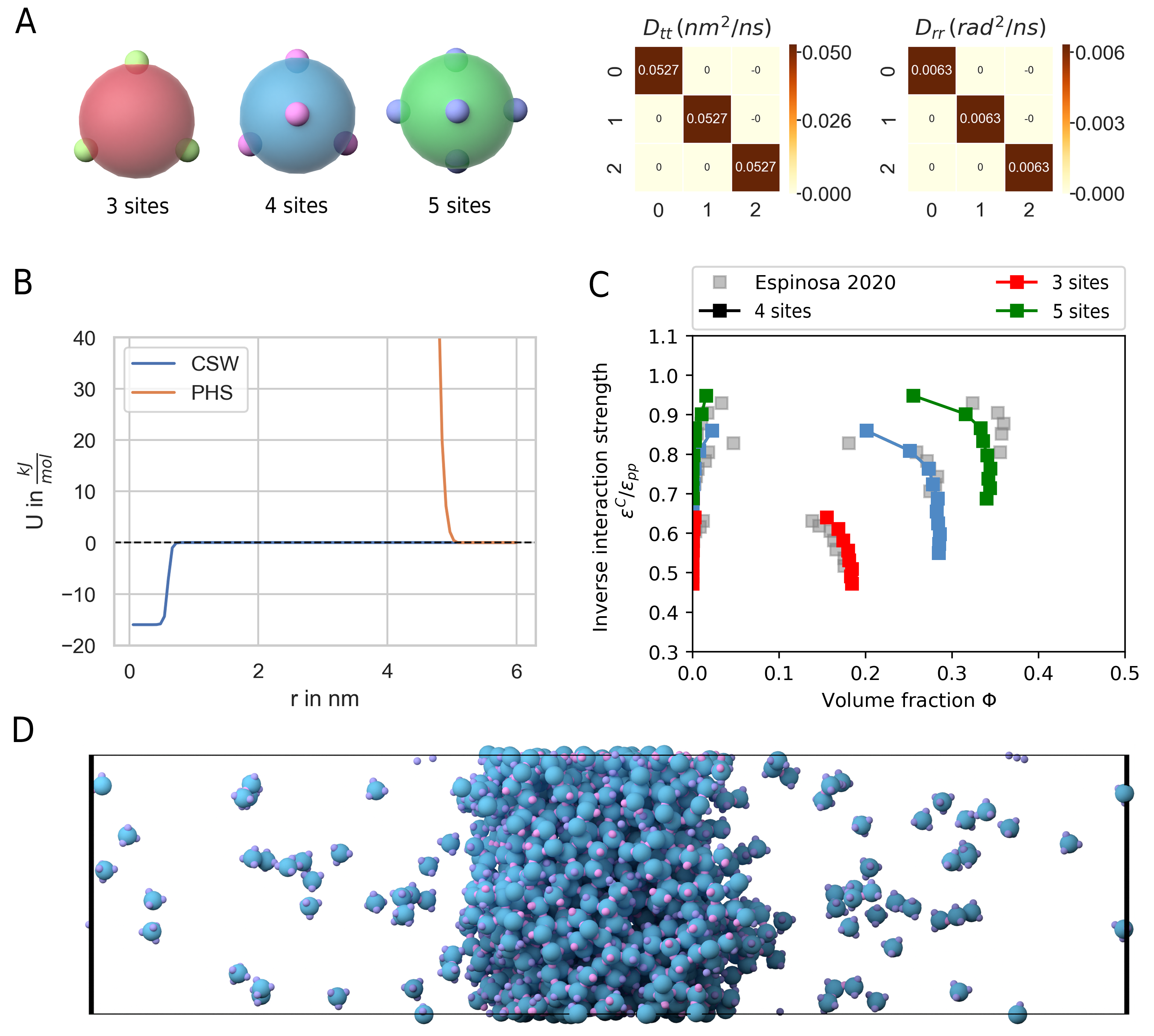
Fig. 33 LLPS of patchy particles. (A) Patchy particles with 3, 4 and 5 sites. Left: The translational and rotational diffusion tensor. (B) Graph of the continuous square-well potential (CSW) used for the attractive patches and the pseudo hard sphere potential (PHS) used for the core particle. (C) Coexistence curves for the 3, 4 and 5 sided patchy particle systems and comparison with the results from Espinosa et al. [90]. (D) Side view showing the dilute and dense phase for the 4-sided patchy particle system.
Benchmarks
To benchmark PyRID I directly compare it to ReaDDy. As a benchmark test I will therefore use the same that has been used in [23]. The system consists of the molecule types A, B and C with radii \(1.5\, nm\), \(3.0\, nm\), and \(3.12\, nm\). The viscosity is set to \(1.0 mPa \cdot s\), which is the value for water at about 293 Kelvin (20°C). The molecules all interact via a harmonic repulsive potential [23]:
where the force constant \(\kappa = 10 kJ/mol\). The interaction distance \(\sigma\) is given by the radii of the interacting molecule pair. In addition, the molecules take part in the reaction \(\ce{A + B <=>[\ce{k_1}][\ce{k_{-1}}] C }\). The rate for the fusion reaction is \(k_1 = 0.001 ns^{-1}\) and the reaction radius \(R_{react} = 4.5 nm\). The fission reaction rate is set to \(k_{-1}=5 \cdot 10^{-5} ns^{-1}\) and the dissociation radius is set equal to \(R_{react}\). The benchmark is carried out for different values of the total initial molecule number \(N_{tot}\), with \(N_A = N_{tot}/4\), \(N_B = N_{tot}/4\), \(N_C = N_{tot}/2\). The number density is, however, kept constant at \(\rho_{tot} = 0.00341 nm^{-3}\) by scaling the simulation box accordingly. Simulations are carried out for \(300 ns\) with an integration time step of \(0.1 ns\). The result of the performance test is shown in Fig. 34 B. For particle numbers between 1.000 and 10.000, the computation time per particle update stays approximately constant at \(1.25 \mu s\), which corresponds to about 800.000 particle updates per second. For particle numbers above 10.000, the performance starts to drop slightly (Fig. 34 B, blue line). The benchmark test has been performed on a machine with an Intel Core i5-9300H with 2.4 GHz and 24 GB DDR4 RAM. Interestingly, PyRID always performed better than ReaDDy for this benchmark test (Fig. 34 B, yellow line). Also, ReaDDy scaled less linear for large particle numbers than PyRID. Shown are the results for ReaDDy ran on the sequential kernel. In addition, I performed the benchmark test for the parallel kernel but the results were always worse. However, in [23], where the same benchmark test has been used, ReaDDy scaled much better and there was almost no performance drop even at 100.000 particles for the sequential kernel (Fig. 34 B, green line). Also, performance increased significantly when using the parallel kernel (down to \(\approx 0.5 \mu s\)). The performance has been tested on a slightly faster but comparable machine with an Intel Core i7 6850K processor at 3.8GHz and 32GB DDR4 RAM. The faster machine is probably the cause for the better performance at particle numbers below 10.000 particles in comparison with my results. However, I can only speculate why ReaDDys’ scaling behavior for large particle numbers is much less linear in my benchmark test and why multi-threading only let to a performance loss. The reason might be that in [23] ReaDDy was compiled for their benchmark system whereas I used the binaries distributed by the developers behind ReaDDy. Nonetheless, the benchmark test shows that PyRIDs performance is very much comparable with ReaDDy, and at least in certain situation PyRID can even outperform ReaDDy. Thereby, for a system with \(10^4\) particles, PyRID is able to perform at \(\approx 80 it/s\) and \(\approx 7\cdot 10^6 /day\). At an integration time step of \(1 ns\), therefore, \(7 ms\) per day can be simulated on medium machine.
Polydispersity
As mentioned in the methods chapter, PyRID uses a hierarchical to efficiently handle polydispersity. As a test, a two component system is used. Both components consist of a single particle. Component A has a radius of \(10\,nm\), component B has a radius of \(2.5\,nm\). The simulation box measures \(75\,nm\cdot 75\,nm\cdot 75\,nm\). The simulation volume is densely packed with both components such that we reach a volume fraction of \(52\%\). The simulation ran for \(1e4\) steps. When not using the hierarchical grid approach but the classical linked cell list algorithm, PyRID only reaches about 80000 particle updates per second (pu/s) on average (Fig. 34 A). However, when using the hierarchical grid, more than 500000 pu/s are reached (Fig. 34 A). If instead of the two component system we only simulate a one component system, PyRID also only reaches about 500000 pu/s (Fig. 34 A). Thereby, PyRID performs similar independent of whether the system is mono- or polydisperse.
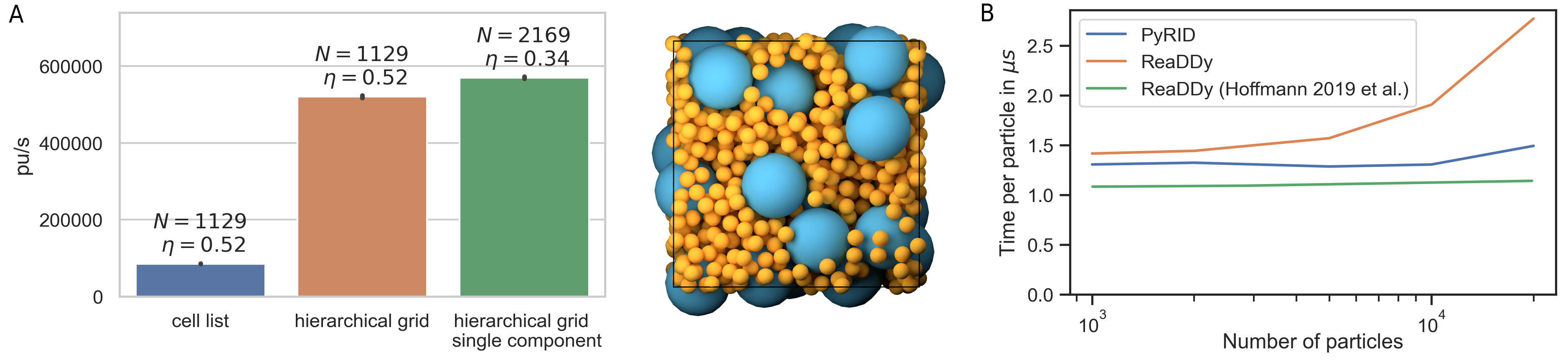
Fig. 34 Performance test of the hierarchical grid approach. (A) Performance hierarchical grid. (B) Performance comparison between PyRID and ReaDDy. On a benchmark system with an Intel Core i5-9300H with 2.4 GHz and 24 GB DDR4 RAM, PyRID (blue line) outperforms ReaDDy (yellow). However, Hoffmann et al. [23] obtained a better performance and especially scaling for ReaDDy on a different machine with an Intel Core i7 6850K processor at 3.8GHz and 32GB DDR4 RAM (green line).