Theory and Methods

In this section, I will introduce and discuss the main methods used in PyRID. I start in section 1.1 Rigid bead molecules by introducing the scheme by which bead molecules are represented. Followed by the derivation of an algorithm for the propagation of translational and predominantly rotational diffusion. The rotational and translational mobility tensors dictate the translational and rotational motion of anisotropic rigid bodies. Therefore, in section 1.3 Mobility tensor for rigid bead models I outline the calculation of the mobility tensors based on a modified Oseen tensor [2]. One of the main features of PyRID that distinguishes it from other molecular dynamics tools such as LAMMPS, Gromacs and HooMD is the ability to simulate arbitrary unimolecular and bimolecular reactions using stochastic simulation algorithms. In section 1.7 Reactions I describe how these reactions are evaluated in PyRID. Another notable feature of PyRID is its ability to restrict the motion of molecules to complex compartment geometries represented by triangulated meshes. Section 1.5 Compartments gives a brief overview of how compartment collisions and surface diffusion are handled. The remainder of this chapter discusses some additional methods and algorithms: Distribution of molecules in mesh volumes and on surfaces, fast data structures for molecular dynamics simulations, fixed concentration boundary conditions and barostat/pressure calculation for rigid bead model systems.

Rigid bead molecules

Proteins and other molecules are not point like particles. Especially the interactions between proteins are not accurately described by isotropic energy potentials. Instead, the physical properties of bio-molecular systems emerge from an-isotropic multivalent interactions [30, 72]. Protein-protein interaction can be accurately simulated in all-atom molecular dynamics simulations. However, even modern computers and algorithms are not efficient enough to simulate systems with more than a few molecules on time scales relevant for processes such as protein assembly and LLPS. Therefore, coarse graining methods are needed [73]. Rigid bead models are a method of minimal coarse graining that have some important benefits. Strong and short ranged interactions between atoms are replaced by a rigid bead topology. This allows for integration time steps several orders larger than in all-atom simulations when atoms within the molecule are held together by an energy potential. Usually, the beads of a rigid bead model do not represent single atoms but pattern the geometry of the molecule of interest [1], significantly reducing the overall number of particles that need to be simulated. In addition, experimentally or theoretically estimated diffusion tensors can be used to accurately describe the diffusive motion of molecules. Importantly, multivalent protein-protein interactions can be described by patches located on the bead model surface. On the downside, the properties of coarse grained model systems strongly depend on the choice of interaction potentials and other model parameters. The estimation of these model parameters is fairly involved and is out of the scope of this work.

The position of each bead i of molecule j can be characterized by

\[\boldsymbol{R}_i(t) = \boldsymbol{R}_{i}^{local}(t) + \boldsymbol{R}_{j}^{O}(t)\]

where

\[\boldsymbol{R}_{i}^{local}(t) = \boldsymbol{A}_j(t) \cdot \boldsymbol{X}_{i}^{local} .\]

Here \(\boldsymbol{X}_{i}^{local}\) are the coordinates of bead i in the local reference frame, and \(\boldsymbol{A}(t)\) and \(\boldsymbol{R}_{j}^{O}(t)\) are the rotation matrix and center of diffusion of molecule j in the lab reference frame respectively. The center of diffusion propagates in response to external forces \(\boldsymbol{F}(t)\) exerted, e.g., by particle-particle interactions or an external force field, and due to hydrodynamic interactions and collisions of the beads with solvent molecules (Brownian motion). Thereby, the total force \(\boldsymbol{F}(t)\) acting on the molecules’ center of diffusion is the sum of all forces \(\boldsymbol{f}_i(t)\) acting on the individual beads:

\[\boldsymbol{F}(t) = \sum_{i = 1}^{N_{beads}}. \boldsymbol{f}_i(t),\]

where \(N_{beads}\) is the total number of beads contained in the molecule.

Propagation of translational and angular motion

The motion of an isolated rigid bead molecule in solution can be described in terms of the Langevin equation for translational and rotational motion. Note that we are always considering isolated molecules in dispersion and do not account for the hydrodynamic interaction between molecules as this is computationally very expensive (\(O(N^2)-O(N^3)\)) [74, 75]. In the most general case the Langevin equation for translational and rotational motion reads [76, 77, 78]:

\[m \frac{d^2\boldsymbol{r}(t)}{dt^2} = \boldsymbol{F} - \Big(\boldsymbol{\Xi}^{tt} \frac{d\boldsymbol{r}}{dt} + \boldsymbol{\Xi}^{tr} \frac{d\boldsymbol{\phi}}{dt}\Big) + \boldsymbol{R}^t\]

\[\frac{d}{dt} \Big( I \frac{d \boldsymbol{\phi}(t)}{dt} \Big) = \boldsymbol{T} - \Big(\boldsymbol{\Xi}^{rr} \frac{d\boldsymbol{\phi}}{dt} + \boldsymbol{\Xi}^{rt} \frac{d\boldsymbol{r}}{dt}\Big) + \boldsymbol{R}^r,\]

where \(\boldsymbol{r}(t)\) is the position of the molecule center and \(\boldsymbol{\phi}(t)\) the rotation angle. \(\boldsymbol{F}\) is the total force exerted on the molecule and \(\boldsymbol{T}\) is the torque. \(\boldsymbol{R}^t\) and \(\boldsymbol{R}^r\) describe the random, erratic movement of the molecule due to collisions with the solvent molecules where

\[\langle \boldsymbol{R}^a(t)\rangle = 0\]

\[\langle R^a_i(t) R^b_j(t')\rangle = 2 k_B T \Xi_{ij}^{ab} \delta(t-t'),\]

with \(a,b \in \{t,r\}\). \(\Xi_{ij}^{ab}\) are the components of the 3 x 3 friction tensors. Here, \(\boldsymbol{\Xi}^{tt}, \boldsymbol{\Xi}^{rr}, \boldsymbol{\Xi}^{tr}, \boldsymbol{\Xi}^{rt}\) are the translational, rotational and translation-rotation coupling friction tensors of the rigid body in the lab frame. Also, \(\boldsymbol{\Xi}^{ab} = k_B T (\boldsymbol{D}^{-1})^{ab}\) (Einstein relation). Due to the translation-rotation coupling, the equations for rotation and translation are not independent. For low-mass particles, such as molecules, and for long enough time intervals, the acceleration of the molecules can be neglected in the description of the diffusion process. As such it is convenient to describe the motion of molecules by overdamped Langevin dynamics also called Brownian motion where \(I \frac{d^2 \phi(t)}{dt^2} = m \frac{d^2 x(t)}{dt^2} = 0\):

\[\frac{d\boldsymbol{r}(t)}{dt} = \boldsymbol{M}^{tt} \boldsymbol{F} + \boldsymbol{M}^{tr} \boldsymbol{T} + \boldsymbol{S}^t\]

\[\frac{d \boldsymbol{\phi}(t)}{dt} = \boldsymbol{M}^{rr} \boldsymbol{T} + \boldsymbol{M}^{rt} \boldsymbol{F} + \boldsymbol{S}^r.\]

with

\[\langle \boldsymbol{S}^a(t)\rangle = 0\]

\[\langle S^a_i(t) S^b_j(t')\rangle = 2 k_B T M_{ij}^{ab} \delta(t-t'),\]

where \(\boldsymbol{M}^{tt}, \boldsymbol{M}^{rr}, \boldsymbol{M}^{tr}, \boldsymbol{M}^{rt}\) are the translational, rotational and translation-rotation coupling mobility tensors of the rigid body in the lab frame and \(\boldsymbol{M}^{ab} = \frac{\boldsymbol{D}^{ab}}{k_B T}\). \(M_{ij}^{ab}\) are the components of the 3 x 3 mobility tensors. Also \(\boldsymbol{M}^{rt} = \boldsymbol{M}^{tr,T}\). In most cases, the effect of the translation-rotation coupling on the molecular dynamics is negligible. However, translation-rotation coupling increases the complexity of the propagation algorithm for the translation and rotation vectors. Therefore, in the following, we will consider translation and rotation as being independent. In this case, the propagator for the Cartesian coordinates as well as the orientation angle can be formulated as [13]

(32)\[\boldsymbol{r}(t) = \boldsymbol{r}(t-\Delta t) + \boldsymbol{A} \boldsymbol{M}^{tt,b} \boldsymbol{A}^T \boldsymbol{F} \Delta t + \boldsymbol{A} \sqrt{2 \boldsymbol{M}^{tt,b} k_B T}\, \boldsymbol{W}^t(\Delta t)\]

(33)\[\boldsymbol{\phi}(t) = \boldsymbol{\phi}(t-\Delta t) + \boldsymbol{A} \boldsymbol{M}^{rr,b} \boldsymbol{A}^T \boldsymbol{T} \Delta t + \boldsymbol{A} \sqrt{2 \boldsymbol{M}^{rr,b} k_B T}\, \boldsymbol{W}^r(\Delta t).\]

Here, \(\boldsymbol{W}(\Delta t)\) is a 3-dimensional Wiener process, i.e. \(\boldsymbol{W}(t+\Delta t) - \boldsymbol{W}(t) \sim \mathcal{N}(0, \Delta t)\), which can be argued from the central limit theorem and the assumption that the forces of the solvent molecules act with equal probability from all directions. The superscript \(b\) indicates that the mobility tensors \(\boldsymbol{M}^{ab,b}\) are given in terms of the body/local frame of the molecule, which is much more convenient when we talk about the propagation algorithm. In this context, \(\boldsymbol{A}\) is the rotation matrix of the molecule. One problem with the rotational equation of motion is that several issues arise depending on how rotations are represented. Propagating the rotation in terms of Euler angles, e.g., will result in numerical drift and singularities [79, 80]. Therefore, especially in computer graphics, it is standard to represent rotations in unit quaternions, which is much more stable and has fewer issues in general. An algorithm for the rotation propagator based on quaternions can, for example, be found in [13]. In the following, I will introduce a more concise derivation of the very same algorithm.

Quaternion propagator

The orientation/rotation of the molecule can be described by a unit quaternion \(\boldsymbol{q} = q_0 + i\,q_1 + j\,q_2 + k\, q_3\) where \(\boldsymbol{q}^2 = \sum_{i=0}^3 q_i^2 = 1\). Quaternions can be thought of as an extension to complex numbers and were introduced in 1844 by Sir William Rowan Hamilton [81]. The rotation quaternion \(\boldsymbol{q}(t)\) propagates in response to the torque \(\boldsymbol{T}_i(t) = \boldsymbol{F}_i(t) \times \boldsymbol{r}_{i}\) exerted by the external forces, where \(\boldsymbol{r}_{i}\) is the distance vector between bead i and the center of diffusion of molecule. The rotation matrix can be represented in terms of rotation quaternions by [79] (pyrid.molecules.rigidbody_util.RBs.calc_orientation_quat):

\[\begin{split}\begin{split}\boldsymbol{A} = \begin{pmatrix} 1-2(q_2^2+q_3^2) & 2(q_1 q_2-q_0 q_3) & 2(q_1 q_3+q_0 q_2) \\ 2(q_1 q_2+q_0 q_3) & 1-2(q_1^2+q_3^2) & 2(q_2 q_3-q_0 q_1) \\ 2(q_1 q_3-q_0 q_2) & 2(q_2 q_3+q_0 q_1) & 1-2(q_1^2+q_2^2) \\ \end{pmatrix}, \end{split}\end{split}\]

The goal is to derive a propagator for the rotation quaternion. A well-established connection between the angular velocity and the unit quaternion velocity is [79]:

(34)\[\frac{d\boldsymbol{q}}{dt} = \frac{1}{2} \frac{d\boldsymbol{\phi}}{dt} \boldsymbol{q} = \boldsymbol{B} \frac{d\boldsymbol{\phi}}{dt}\]

where

\[\begin{split}\begin{split}\boldsymbol{B} = \frac{1}{2} \begin{pmatrix} -q_1 & -q_2 & -q_3 \\ q_0 & q_3 & -q_2 \\ -q_3 & q_0 & q_1 \\ q_2 & -q_1 & q_0 \\ \end{pmatrix}. \end{split}\end{split}\]

Inserting (33) into (34), we get:

(35)\[\boldsymbol{q}(t) = \boldsymbol{q}(t-\Delta t) + \boldsymbol{B}\boldsymbol{A} \boldsymbol{M}^{rr,b} \boldsymbol{A}^T \boldsymbol{T} \Delta t + \boldsymbol{B} \boldsymbol{A} \sqrt{2 \boldsymbol{M}^{rr,b} k_B T}\, \boldsymbol{W}^r(\Delta t).\]

The factor \(\boldsymbol{B}\boldsymbol{A}\) can, however, be simplified:

\[\begin{split}\begin{split} \boldsymbol{B}\boldsymbol{A} = & \frac{1}{2} \begin{pmatrix} -q_1 & -q_2 & -q_3 \\ q_0 & q_3 & -q_2 \\ -q_3 & q_0 & q_1 \\ q_2 & -q_1 & q_0 \\ \end{pmatrix} \begin{pmatrix} 1-2(q_2^2+q_3^2) & 2(q_1 q_2-q_0 q_3) & 2(q_1 q_3+q_0 q_2) \\ 2(q_1 q_2+q_0 q_3) & 1-2(q_1^2+q_3^2) & 2(q_2 q_3-q_0 q_1) \\ 2(q_1 q_3-q_0 q_2) & 2(q_2 q_3+q_0 q_1) & 1-2(q_1^2+q_2^2) \\ \end{pmatrix}\\ = & \frac{1}{2} \begin{pmatrix} -q_1 & -q_2 & -q_3 \\ q_0 & q_3 (1-2 q^2 ) & q_2 (2 q^2 -1) \\ q_3 (2 q^2 -1) & q_0 & q1 (1-2 q^2 ) \\ q_2 (1-2 q^2) & q_1 (2 q^2-1) & q_0 \\ \end{pmatrix} \\ = & \frac{1}{2} \begin{pmatrix} -q_1 & -q_2 & -q_3 \\ q_0 & -q_3 & q_2 \\ q_3 & q_0 & -q_1 \\ -q_2 & q_1 & q_0 \\ \end{pmatrix}, \end{split}\end{split}\]

where \(q^2 = q_0^2+q_1^2+q_2^2+q_3^2 = 1\). For the quaternion to accurately represent the rotation, we need to ensure that it keeps its unit length. However, due to the finite time step in simulations, the quaternion will diverge from unit length over time. Thus, it is necessary to frequently re-normalize the quaternion. Ilie et al. [13] point out that re-normalization will introduce a bias by changing the sampled phase space distribution. Thereby, it is more appropriate to introduce a constraint force using the method of undetermined Lagrange multipliers as is used in molecular dynamics algorithms such as SHAKE. However, for integration time steps used in practice, I found the error introduced by re-normalization to be negligible. Validation of the above algorithms are presented in section Anisotropic diffusion.

Mobility tensor for rigid bead models

In order simulate the motion of molecules with the algorithms introduced above, we need to calculate the molecule’s diffusion tensor. Diffusion tensors have also been estimated experimentally [14] or using molecular dynamics simulations [82]. However, for many proteins, the diffusion tensor is unknown. Therefore, it would often be more convenient to calculate the diffusion tensor directly from the coarse-grained representation of a molecule in terms of the rigid bead model. Pioneering work in this direction has been done by Bloomfield et al. [83] and Torre and Bloomfield [18]. In the following I will only present the main results that are needed for the calculation of the rigid bead model diffusion tensor. For the interested reader, a more in depth introduction can be found in Appendix A Appendix A.

In general, the mobility and/or diffusion tensor of an anisotropic rigid body can be calculated from the inverse of the rigid body’s friction supermatrix [2]:

(36)\[\begin{split}\begin{pmatrix} \boldsymbol{M}^{tt} & \boldsymbol{M}^{tr} \\ \boldsymbol{M}^{rt} & \boldsymbol{M}^{rr} \\ \end{pmatrix} = \frac{1}{k_B T} \begin{pmatrix} \boldsymbol{D}^{tt} & \boldsymbol{D}^{tr,T} \\ \boldsymbol{D}^{rt} & \boldsymbol{D}^{rr} \\ \end{pmatrix} = \begin{pmatrix} \boldsymbol{\Xi}^{tt} & \boldsymbol{\Xi}^{tr} \\ \boldsymbol{\Xi}^{rt} & \boldsymbol{\Xi}^{rr} \\ \end{pmatrix}^{-1}.\end{split}\]

Therefore, the main challenge lies in deriving an expression for the translational, rotational and translation-rotation coupling tensors of the friction super matrix \(\boldsymbol{\Xi}^{tt}, \boldsymbol{\Xi}^{rr}, \boldsymbol{\Xi}^{tr}=\boldsymbol{\Xi}^{rt,T}\). PyRID uses a method based on a modified Oseen tensor [2, 18] to account for the hydrodynamic interaction between the beads of a rigid bead molecule in a first order approximation [16]. For a rigid molecule consisting of \(N\) different beads, the friction tensors read

(37)\[\begin{split}\begin{split} &\boldsymbol{\Xi}^{tt} = \sum_{i=1}^N \sum_{j=1}^N \boldsymbol{\xi}_{ij}^{tt} \\ &\boldsymbol{\Xi}_{O}^{tr} = \sum_{i=1}^N \sum_{j=1}^N ( -\boldsymbol{\xi}_{ij}^{tt} \cdot \boldsymbol{A}_j + \boldsymbol{\xi}_{ij}^{tr} ) \\ &\boldsymbol{\Xi}_{O}^{rt} = \sum_{i=1}^N \sum_{j=1}^N ( \boldsymbol{A}_j \cdot \boldsymbol{\xi}_{ij}^{tt} + \boldsymbol{\xi}_{ij}^{rt} ) \\ &\boldsymbol{\Xi}_{O}^{rr} = \sum_{i=1}^N \sum_{j=1}^N ( \boldsymbol{\xi}_{ij}^{rr} - \boldsymbol{\xi}_{ij}^{rt} \cdot \boldsymbol{A}_j + \boldsymbol{A}_i \cdot \boldsymbol{\xi}_{ij}^{tr} - \boldsymbol{A}_i \cdot \boldsymbol{\xi}_{ij}^{tt} \boldsymbol{A}_j) \end{split}.\end{split}\]

Here \(\boldsymbol{A}\) is given by

\[\begin{split}\boldsymbol{A}_i = \begin{pmatrix} 0 & -z_i & y_i \\ z_i & 0 & -x_i \\ -y_i & x_i & 0 \\ \end{pmatrix}\end{split}\]

with \(\boldsymbol{r}_i = x_i e_x + y_i e_y +z_i e_z\) being the position vector of bead i in the molecule’s local reference frame. \(\boldsymbol{\xi}^{ab}, a,b \in \{t,r\}\) are the translational, rotational and translation-rotation coupling friction tensors of the system of \(N\) freely diffusing beads. \(\boldsymbol{\xi}\), are calculated from the inverse of the mobility supermatrix [16]:

(38)\[\begin{split}\begin{pmatrix} \boldsymbol{\xi}^{tt} & \boldsymbol{\xi}^{tr} \\ \boldsymbol{\xi}^{rt} & \boldsymbol{\xi}^{rr} \\ \end{pmatrix} = \begin{pmatrix} \boldsymbol{\mu}^{tt} & \boldsymbol{\mu}^{tr} \\ \boldsymbol{\mu}^{rt} & \boldsymbol{\mu}^{rr} \\ \end{pmatrix}^{-1}\end{split}\]

Here \(\boldsymbol{\xi}^{ab}\) are of dimension (3Nx3N), forming the friction supermatrix of dimension (6N,6N). \(\boldsymbol{\mu}^{ab}\) are the (3Nx3N) dimensional elements of the mobility supermatrix. The translational mobility tensor \(\boldsymbol{\mu}^{tt}\) for a system of different sized beads is, in first order approximation, given by [16]:

(39)\[\begin{split}\begin{split} \boldsymbol{\mu}^{tt}_{ij} = & \delta_{ij} (6 \pi \eta_0 \sigma_i)^{-1} \boldsymbol{I} + (1-\delta_{ij})(8 \pi \eta_0 r_{ij}^{-1})(\boldsymbol{I}+\boldsymbol{P}_{ij}) \\ & + (8 \pi \eta_0 r_{ij}^{-3})(\sigma_i^2+\sigma_j^2)(\boldsymbol{I}-3 \boldsymbol{P}_{ij}), \end{split}\end{split}\]

where \(\boldsymbol{P}_{ij} = \Big(\boldsymbol{I}+\frac{\boldsymbol{r} \otimes \boldsymbol{r}}{r^2} \Big)\), \(\eta_0\) is the fluid viscosity and \(r_{ij}\) is the distance vector between bead i and bead j. \(\boldsymbol{I}\) is the identity matrix. The mobility tensor for rotation, however, not accounting for the bead radii in the hydrodynamic interaction term, is given by [16]:

(40)\[\begin{split}\begin{split} \boldsymbol{\mu}^{rr}_{ij} = & \delta_{ij} (8 \pi \eta_0 \sigma_i^3)^{-1} \boldsymbol{I} \\ & + (1 - \delta_{ij})(16 \pi \eta_0 r^3_{ij})^{-1} (3 \boldsymbol{P}_{ij} - \boldsymbol{I}). \end{split}\end{split}\]

In this formulation, there is still a correction for the bead radii missing. This correction consists of adding \(6 \eta_0 V_m \boldsymbol{I}\) to the diagonal components of the rotational friction tensor \(\boldsymbol{\Xi}^{rr}_O\), where \(V_m\) is the total volume of the rigid bead molecule [16, 20]. The rotation-translation coupling is given by [16]:

(41)\[\boldsymbol{\mu}^{rt}_{ij} = (1-\delta_{ij}) (8 \pi \eta_0 r_{ij}^2)^{-1} \boldsymbol{\epsilon}\boldsymbol{\hat{r}}_{ij},\]

where \(\epsilon\) is the Levi-Civita symbol with [19]

\[\begin{split}\epsilon \cdot \boldsymbol{r}_{ij} = \begin{pmatrix} 0 & z_{ij} & -y_{ij} \\ -z_{ij} & 0 & x_{ij} \\ y_{ij} & -x_{ij} & 0 \\ \end{pmatrix}.\end{split}\]

\(\boldsymbol{\mu}^{tt}, \boldsymbol{\mu}^{rr}, \boldsymbol{\mu}^{rt}\) describe the mobility of a multi-sphere system with hydrodynamic interactions. From the above follows that we need to calculate the inverse of a supermatrix twice, once in equation (36) and once in equation (37). A super Matrix \(\boldsymbol{M}=[[\boldsymbol{M}_1, \boldsymbol{M}_2], [\boldsymbol{M}_3, \boldsymbol{M}_4]]\) is invertible, if both the diagonal blocks, \(\boldsymbol{M}_1\) and \(\boldsymbol{M}_4\) are invertible The inverse of a (2x2) supermatrix can be calculated by [21], [22]:

(42)\[\begin{split}\begin{split} & \boldsymbol{T}_1 = (\boldsymbol{M}_1 - \boldsymbol{M}_2 \boldsymbol{M}_4^{-1} \boldsymbol{M}_3)^{-1} \\ & \boldsymbol{T}_2 = -\boldsymbol{M}_1^{-1} \boldsymbol{M}_2 (\boldsymbol{M}_4-\boldsymbol{M}_3 \boldsymbol{M}_1^{-1} \boldsymbol{M}_2)^{-1} \\ & \boldsymbol{T}_3 = -\boldsymbol{M}_4^{-1} \boldsymbol{M}_3 (\boldsymbol{M}_1-\boldsymbol{M}_2 \boldsymbol{M}_4^{-1} \boldsymbol{M}_3)^{-1} \\ & \boldsymbol{T}_4 = (\boldsymbol{M}_4 - \boldsymbol{M}_3 \boldsymbol{M}_1^{-1} \boldsymbol{M}_2)^{-1} \\ \end{split}\end{split}\]

Center of Diffusion

One problem that arises with the above description is that we have not yet formulated an expression for the center of diffusion of the rigid bead molecule. For a rigid body immersed in a fluid, the force and torque act at the body’s center of diffusion [15], which, in general, is different from the center of mass except for spherically symmetric molecules. The center of diffusion can, however, be calculated from a diffusion tensor referring to an arbitrary origin by [2]

(43)\[\begin{split}\begin{split} \boldsymbol{r}_{OD} = & \begin{pmatrix} x_{OD} \\ y_{OD}\\ z_{OD} \end{pmatrix} \\ = & \begin{pmatrix} D_{rr}^{yy}+D_{rr}^{zz} & -D_{rr}^{xy} & -D_{rr}^{xz}\\ -D_{rr}^{xy} & D_{rr}^{xx}+D_{rr}^{zz} & -D_{rr}^{yz}\\ -D_{rr}^{xz} & -D_{rr}^{yz} & D_{rr}^{yy}+D_{rr}^{xx} \end{pmatrix}^{-1} \begin{pmatrix} D_{tr}^{zy}-D_{tr}^{yz}\\ D_{tr}^{xz}-D_{tr}^{zx}\\ D_{tr}^{yx}-D_{tr}^{xy} \end{pmatrix} \end{split}.\end{split}\]

Compartments

Compartmentalization plays an important role in cell processes. Therefore, we would like to be able to restrict diffusion and reactions to the volume and surface of arbitrarily shaped compartments. There exist different methods to restrict the motion of particles to a confined region. One option is to pattern the boundary of the compartment with particles such that they interact with the particle inside the compartment via a repulsive interaction potential. This method, however, has several downsides. On the one hand, one needs many particles to pattern the surface, which makes this method highly inefficient. On the other hand this method does not support surface diffusion in a straight forward way. Another approach would be to add external potentials/force fields that restrict the motion of particles either to the volume or the surface of a compartment. This method is used in ReaDDy [23]. However, complex geometries/compartment shapes are more difficult to establish. A third approach is to represent the compartment geometry by triangulated meshes as is done, e.g. in MCell [10]. This approach has several benefits over alternative approaches, such as representing compartments by force fields or other particles. Triangulated meshes are heavily used in computer graphics. Therefore, a large number of highly optimized algorithms exist. Also, triangulated meshes are very well suited to represent complex compartment geometries. In the following, I will introduce how PyRID handles surface diffusion and collisions of particles with compartment surfaces.

Triangulated meshes

A triangulated mesh surface is described by a set of \(N\) vertices. These vertices are combined to sets of \(n\) vertices that form the mesh faces. In our case, each face is a triangle (\(n=3\)) determined by three vertices \(\boldsymbol{p}_i, \boldsymbol{p}_j\) and \(\boldsymbol{p}_k\). The order in which these vertices are sorted per triangle determines the orientation of the triangle normal vector. The normal vector of the triangle plane is given by \(\boldsymbol{n} = (\boldsymbol{p}_1-\boldsymbol{p}_0)\times(\boldsymbol{p}_2-\boldsymbol{p}_0)\). In the following, I will write the three vertices of a triangle as \(\boldsymbol{p}_0, \boldsymbol{p}_1\) and \(\boldsymbol{p}_2\) and vertices are always sorted in counter clockwise order (Fig. 15 B). Thereby, the normal vector of a triangle points outside the mesh compartment. In PyRID, a compartment is defined by a triangulated manifold mesh, which is a mesh without holes and disconnected vertices or edges, i.e. it has no gaps and separates the space on the inside of the compartment from the space outside [34]. As one vertex is shared by at minimum three triangles it is most convenient to store meshes in a shared vertex mesh data structure [34] where an array with all vertex position vectors is kept as well as an array holding for each triangle the indices of the three vertices that make up the triangle (Fig. 15 A).

Volume molecules

The collision response of a molecule with the mesh is calculated in two different ways. For large rigid bead molecules, each triangle exerts a repulsive force on the individual beads; for small, isotropic molecules or atoms, a ray tracing algorithm is used.

Contact forces

Contact detection generally consists of two phases, 1) neighbor searching and 2) contact resolution. Contact detection and update of contact forces can become fairly involved, depending on the required accuracy, the surface complexity, the type of geometries involved, and whether frictional forces need to be accounted for. Contact resolution of the more complex type is found primarily in discrete element method simulations [84]. Here, however, we will not require exact accuracy but instead use a simple but, as I think, sufficiently accurate approach. A bead \(i\) is said to be in contact with a mesh element \(j\) (which can be a vertex, edge, or face) if the minimum distance \(r_{ij}\) is smaller than the bead radius. In this case, a repulsive force is exerted on the bead:

\[U_{wall, i} = \sum_j^N \frac{k}{2} (r_{ij}-d)^2 \Omega_{ij}.\]

, where \(k\) is the force constant, \(d\) is the bead radius, and \(N\) is the number of faces that are in contact with bead \(i\). In general, \(\Omega_{ij}\) accounts for the amount of overlap of bead \(i\) with mesh face \(j\). However, calculation of \(\Omega_{ij}\) is computationally expensive. Therefore, we here use a simple approximation \(\Omega_{ij} = 1/N\) with \(N = |\mathcal{F}|\) where \(\mathcal{F}\) is the set of all faces the bead is in contact with. Thereby, we assume that the bead overlaps by the same amount with each mesh element and only account for overlaps with faces as valid contacts but not edges or vertices. If \(\mathcal{F} = \emptyset\), only the distance to the closest mesh element is used to calculate the repulsive force, which in this case is either an edge or a vertex. To calculate the distance between the bead and a triangle, PyRID uses the “Point to Triangle” algorithm by Eberly [9].

Ray tracing

Contact force calculations are disadvantageous for small, spherical molecules because they require a very small integration time step. Here, ray tracing is more convenient as it works independently of the chosen integration time step. In this approach, which is similar to the contact detection used in MCell [10], the displacement vector \(\boldsymbol{\Delta R}\) of the molecule is traced through the simulation volume and collisions with the compartment boundary (the mesh) are resolved via reflection.

\[\boldsymbol{\Delta R}_{refl} = \boldsymbol{\Delta R} - 2 (\boldsymbol{\Delta R} \cdot \hat{\boldsymbol{n}}) \hat{\boldsymbol{n}},\]

where \(\hat{\boldsymbol{n}}\) is the normal vector of the triangle face. Collision tests are done using the “Fast Voxel Traversal Algorithm for Ray Tracing” introduced by Amanatides and Woo [5].

Surface molecules

Surface molecules laterally diffuse within the mesh surface and can represent any transmembrane molecules such as receptors. Here, I take a similar approach to MCell. Thereby, a molecule diffuses in the plane of a triangle until it crosses a triangle edge. In this case, the molecule’s displacement vector \(\Delta R\) is advanced until that edge and then rotated into the plane of the neighboring triangle where the rotation axis is given by the shared triangle edge. Thereby, the molecule will move in a strait line on the mesh surface (Fig. 15 C-E). This method is equivalent to unfolding the triangles over the shared edge such that they end up in a common tangent space, i.e. such that they are co-planar, advancing the position vector, and folding/rotating back. From the latter method it becomes intuitively clear that the molecule will indeed move in a straight line on the mesh surface. In the following I will introduce the details of the method sketched above.

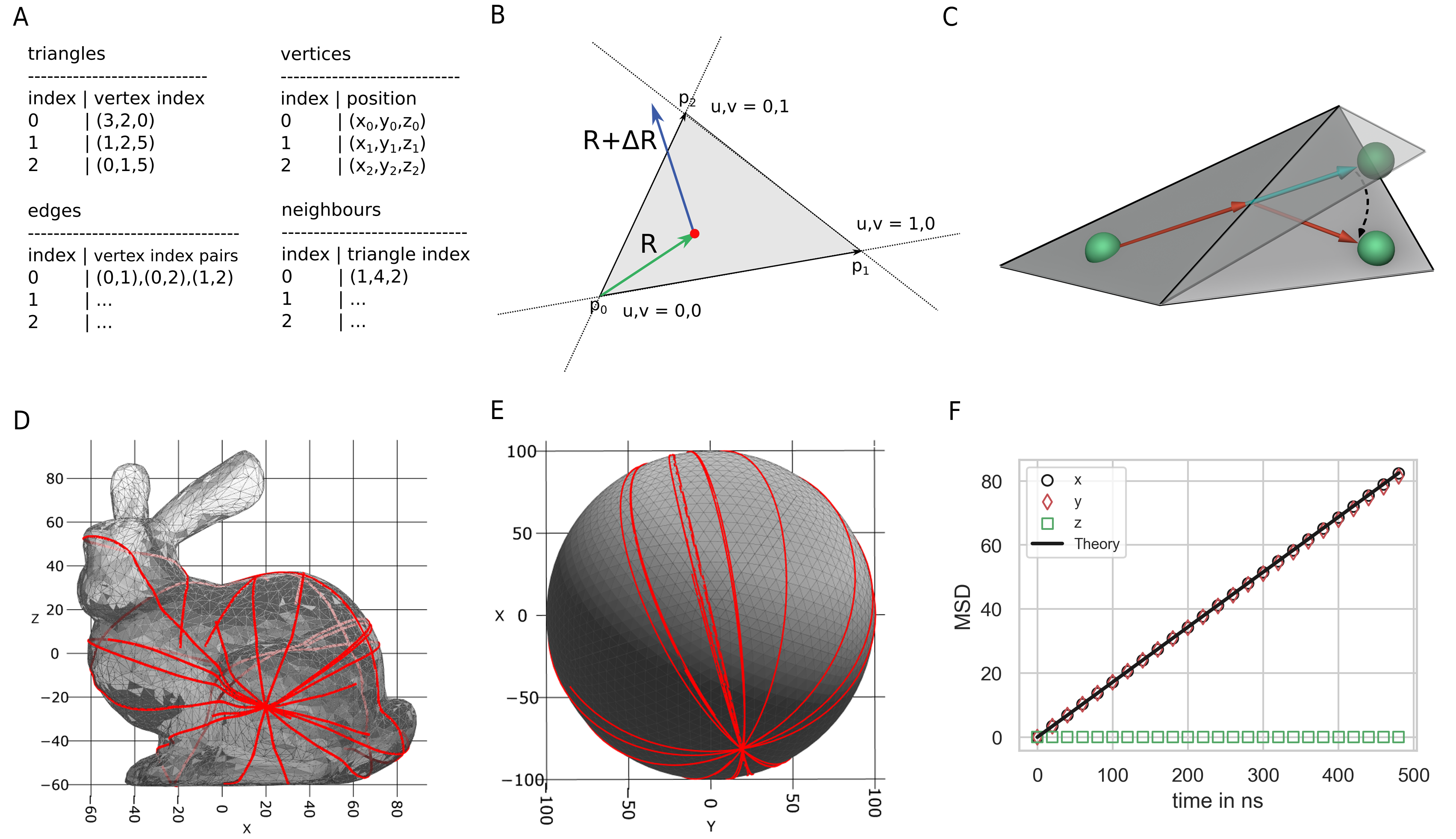
../../_images/Fig_Geodesics.png — Fig. 15 **Mesh compartments and surface molecules.** **(A)** PyRID uses triangulated meshes to represent compartments. These are kept in a shared vertex mesh data structure (top left, right) [34]. In addition, for neighbour search, two array that hold for each triangle the vertex indices of the three triangle edges and the triangle indices of the three triangle neighbours are used. **(A)** Triangle vertices belonging to a triangle are ordered counterclockwise, as are edges. Efficient algorithms based on barycentric triangle coordinates are used to check whether a point lies within a triangle or whether a displacement vector intersects a triangle edge. **(A)** Visualization of mesh surface ray marching. If a molecule (green sphere) crosses a triangle edge, its displacement vector is advanced to the corresponding edge and then rotated into the plane of the neighboring triangle. **D,E** By the ray marching method described in the text, molecules follow a geodesic paths on the mesh surface. F The mean squared displacement of diffusing surface molecules is in agreement with theory. According to theory, in 2 dimensions \(MSD = 4Dt\). In this validation example, \(D=43 nm^2/\mu s\).

Surface ray marching

First, we need to be able to detect if a triangle edge has been crossed, and to which neighbouring triangle this edge belongs. Therefore, in addition to the triangle and vertex data, for each triangle, the vertex indices of the three triangle edges are kept in an array (Fig. 15 A). Edges are sorted in counter clockwise order. Also, for each of the three edges the index of the corresponding neighbouring triangle is kept in a separate array for fast lookup (Fig. 15 A).

The triangle edge intersection test can be made efficient by the use of barycentric coordinates. Let \(\boldsymbol{p}_0, \boldsymbol{p}_1, \boldsymbol{p}_2\) be the three vertices of a triangle. Also, the vertices are numbered in counter clockwise order and the triangle origin is at \(\boldsymbol{p}_0\). Then, the center of the molecule \(R_0\) can be described in barycentric coordinates by

(44)\[\boldsymbol{R}_0 = \boldsymbol{p}_0 + u(\boldsymbol{p}_1-\boldsymbol{p}_0) + v (\boldsymbol{p}_2-\boldsymbol{p}_0),\]

and the molecule displacement vector by

\[\boldsymbol{\Delta R} = du(\boldsymbol{p}_1-\boldsymbol{p}_0) + dv (\boldsymbol{p}_2-\boldsymbol{p}_0),\]

Efficient algorithms to compute the barycentric coordinates \(u\) and \(v\) can, e.g., be found in [6]. The triangle edges are sorted in counter clockwise order, starting from the triangle origin \(\boldsymbol{p}_0\). As such, we are on the line \(\boldsymbol{p}_0 + u(\boldsymbol{p}_1-\boldsymbol{p}_0)\) (edge 0) if \(v=0\), on the line \(\boldsymbol{p}_0 + v (\boldsymbol{p}_2-\boldsymbol{p}_0)\) (edge 2) if \(u = 0\) and on the line \(u \boldsymbol{p}_1 + v \boldsymbol{p}_2\) (edge 1) if \(u+v=1\). Thereby, the edge intersection test comes down to solving

(45)\[\begin{split}\begin{split} & u+t_{1}\cdot du = 0 \\ & v+t_{0}\cdot dv = 0 \\ & (u+t_{2} \cdot du) + (v+t_{2} \cdot dv) = 1 , \end{split}\end{split}\]

where \(t_{i}\) with \(i \in \{0,1,2\}\) is the distances to the respective edge \(i\) along the displacement vector. We find that the intersections occur at

(46)\[\begin{split}\begin{split} & t_{1} = -\frac{u}{du} \,\, (\text{edge 1}) \\ & t_{0}=-\frac{v}{dv} \,\, (\text{edge 0})\\ & t_{2}=\frac{1-u-v}{du+dv} \,\, (\text{edge 2}) . \end{split}\end{split}\]

To determine with which edge \(\boldsymbol{R}+\boldsymbol{\Delta R}\) intersects first, we simply need to check for the smallest positive value of \(t_{i}\). Afterward, we advance \(\boldsymbol{R}\) to the intersecting edge, reduce \(\boldsymbol{\Delta R}\) by the corresponding distance traveled and transform \(\boldsymbol{R}\) to the local coordinate frame of the neighboring triangle. At last, \(\boldsymbol{\Delta R}\) is rotated into the plane of the neighboring triangle. This can be done efficiently using Rodrigues’ rotation formula

(47)\[\Delta \boldsymbol{R}_{rot} = \Delta \boldsymbol{R} \cos(\phi) + (\boldsymbol{a}_n \times \Delta \boldsymbol{R}) \sin(\phi) + \boldsymbol{a}_n (\boldsymbol{a}_n \cdot \Delta \boldsymbol{R}) (1-\cos(\phi)),\]

where

(48)\[\begin{split}\begin{split} & \cos(\phi) = \frac{\hat{\boldsymbol{n}}_1 \cdot \hat{\boldsymbol{n}}_2}{|\hat{\boldsymbol{n}}_1| |\hat{\boldsymbol{n}}_2|} \\ & \sin(\phi) = \frac{\hat{\boldsymbol{n}}_1 \times \hat{\boldsymbol{n}}_2}{|\hat{\boldsymbol{n}}_1| |\hat{\boldsymbol{n}}_2|} \end{split}.\end{split}\]

Here, \(\hat{\boldsymbol{n}}_1\) and \(\hat{\boldsymbol{n}}_2\) are the normal vectors of the two neighboring triangles. As PyRID supports anisotropic rigid bead molecules, the orientation of the molecule needs to be updated as well for each triangle that is crossed. It is not sufficient, however, to rotate the molecule only after it has reached its final position, because the final orientation depends on the exact path that is taken (in case multiple triangles are crossed) and not only on the normal vector/orientation of the target triangle plane. The rotation quaternion is given by:

(49)\[\boldsymbol{q} = \cos(\phi/2) + \boldsymbol{a}_{n} \sin(\phi/2),\]

where \(\sin(\phi/2)\) and \(\cos(\phi/2)\) can be calculated from the half-angle formulas for sine and cosine such that the \(\cos(\phi)\) and \(\sin(\phi)\) that were calculated to rotate \(\Delta R\) can be reused. The molecule’s orientation quaternion is than propagated by quaternion multiplication. The procedure is stopped if \(\boldsymbol{R}_0 +\Delta \boldsymbol{R}\) end up inside the triangle the molecule is currently located on, i.e. if \(0<=u<=1, 0<=v<=1, u+v<=1\).

Integrating the equation of motion

Because in PyRID the mobility of each molecule is described by the mobility tensor in the local frame instead of a scalar mobility coefficient, integrating the equation of motion for surface molecules becomes straight forward. Here, we can simply skip the z components in the integration scheme (Eqs.(32), (35)). Otherwise, we would need to calculate the tangent external and Brownian force vectors.

Boundary Conditions

PyRID supports three kinds of boundary conditions:

Periodic,
repulsive and
fixed concentration boundary conditions.

Repulsive boundary conditions are handled either by a repulsive interaction potential or via ray tracing, depending on the molecule type (see section 1.5.2 Volume molecules). For periodic boundary conditions, the minimal image convention is applied (Fig. 10 C). Thereby, each particle only interacts with the closest image of the other particles in the system. Note, however, that the box size must not become too small, otherwise particles start to interact with themselves. As periodic and repulsive boundary conditions are very common, I will, in the following only introduce the fixed concentration boundary conditions in more detail, which is a feature unique to PyRID.

Fixed concentration boundary conditions

Fixed concentration boundary conditions couple the simulation box to a particle bath. Thereby, we can simulate, e.g., a sub-region within a larger system without the need to simulate the dynamics of the molecules outside simulation box directly. Instead, molecules that are outside the simulation box are treated as ’virtual’ molecules that only become part of the simulation if they cross the simulation box boundary. In PyRID it is possible to have mesh compartments intersect with the simulation box boundary. Molecules then enter and exit the simulation across the intersection surface or the intersection line in the case of surface molecules.

Each iteration of a simulation, the expected number of hits between a molecule type and simulation box boundaries are calculated. The number of hits depends on the outside concentration of the molecule, the diffusion coefficient and the boundary surface area. The average number of volume molecules that hit a boundary of area \(A\) from one side within a time step \(\Delta t\) can be calculated from the molecule concentration \(C\) and the average distance a diffusing molecule travels normal to a plane \(l_{n}\) within \(\Delta t\) [10]:

\[N_{hits} = \frac{A l_{n}}{2 C},\]

where

\[l_{n} = \sqrt{\frac{4D\Delta t}{\pi}}.\]

Here \(D = Tr(\boldsymbol{D}^{tt,b})/3\) is the scalar translational diffusion coefficient. For surface molecules \(D = Tr(\boldsymbol{D}_{xy}^{tt,b})/2\) and

\[N_{hits} = \frac{L l_{n}}{2 C},\]

where \(L\) is the length of the boundary edge. The boundary crossing of molecules can be described as a Poisson process. As such, the number of molecules that cross the boundary each time step is drawn from a Poisson distribution with a rate \(N_{hits}\).

The normalized distance that a crossing molecule ends up away from the plane/boundary follows distribution [10]:

\[P(d\tilde{x}) = 1-e^{-d\tilde{x}^2}+\sqrt{\pi}*dx*\text{erfc}(d\tilde{x})\]

The distance vector normal to the plane after the crossing can then be calculated from the diffusion length constant \(\lambda\) and the plane’s normal vector \(\hat{\boldsymbol{n}}\) by \(d\boldsymbol{x} = \lambda \, d\tilde{x} \, \hat{\boldsymbol{n}} = \sqrt{4Dt} \, d\tilde{x} \, \hat{\boldsymbol{n}}\).

In the case that a molecule enters the simulation box close to another boundary, e.g. of a mesh compartment, we may also want to account for the distance traveled parallel to the plane in order to correctly resolve collision with the mesh. However, currently PyRID does not account for this. For small integration time steps and meshes that are further than \(\sqrt{4Dt}\) away from the simulation box boundary, the error introduced should, however, be negligible.

Now that the number of molecules and their distance away from the plane are determined, the molecules are distributed in the simulation box. Since the diffusion along each dimension is independent we can simply pick a random point uniformly distributed on the respective plane. For triangulated mesh surfaces, triangles are picked randomly, weighted by their area. Sampling a uniformly distributed random point in a triangle is done by [26]

\[P(\boldsymbol{r}) = (1-\sqrt{\mu_1})*\boldsymbol{p}_0+(\sqrt{\mu_1}*(1-\mu_2))*\boldsymbol{p}_1+(\mu_2*\sqrt{\mu_1})*\boldsymbol{p}_2 ,\]

where \(\mu_1, \mu_2\) are random numbers between 0 and 1. \(\boldsymbol{p}_0, \boldsymbol{p}_1, \boldsymbol{p}_2\) are the three vertices of the triangle.

Note that, in general, any interactions between the virtual molecules are not accounted for. Therefore, fixed concentration boundary conditions only result in the same inside and outside concentrations if no molecular interactions are simulated.

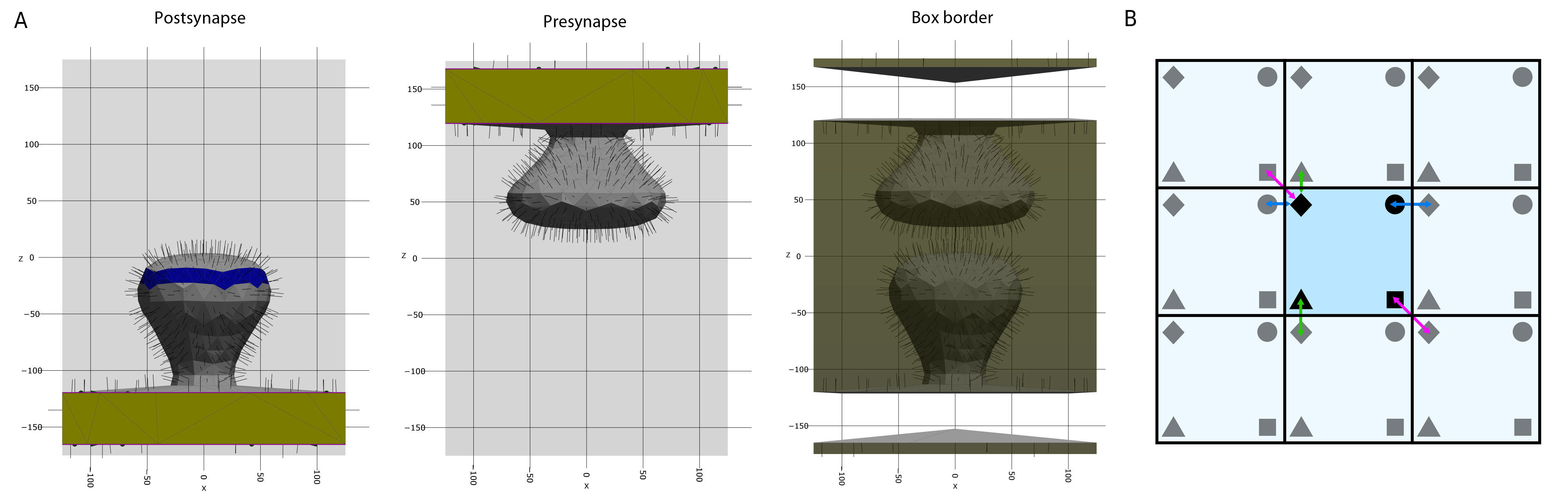
../../_images/Boundaries.png — Fig. 16 **Boundaries.** A (left, middle) In PyRID, the user can define different face groups. Face groups can be used, e.g., to distribute molecules on specific regions of the mesh surface (blue). When a compartment intersects with the simulation box, the intersecting triangles are assigned to a transparent class (yellow), as are the corresponding edges that intersect with the boundary (purple lines). If boundary conditions are set to “fixed concentration” transparent triangles and edges act as absorbing boundaries but in addition release new molecules into the simulation volume. (Right) If mesh compartments intersect the boundary of the simulation box, the remaining part of the box boundary must also be represented by a triangulated mesh. B For periodic boundary conditions, PyRID follows the minimal image convention, i.e. a particle (black marker) only interacts (colored arrows) with the closest image (grey marker) of the other particles in the system.

Reactions

In this section, methods to simulate reactions between proteins and other molecules are introduced. Reactions include, for example, post-translational modifications such as phosphorylation or ubiquitination or binding of ligands and ATP. This list could be continued. In PyRID, reactions are described on several different levels. As a result of rigid bead molecules consisting of one or several subunits, reactions can be defined either on the molecule level or on the bead/particle level. In addition, reactions are categorized into bi-molecular (second order) and uni-molecular (first order) and zero order reactions. Each uni- and bimolecular reaction can consist of several different reaction paths, each belonging to a different reaction type (for an overview see Fig. 17). Uni-molecular reactions are divided into the following categories:

decay reactions,
fission reactions,
conversion reactions.

Decay reactions account for the degradation of proteins whereas fission reactions can be used to describe ligand unbinding but also, e.g., the disassembly of protein complexes or even the flux of ions in response to ion channel opening. Conversion reactions on the other hand may be used to describe different folded protein states that change the protein properties, post-translational modifications but also binding and unbinding reactions in the case where we do not need to model the ligands explicitly (which is the case, e.g. if we can assume an infinite ligand pool). Bi-molecular reactions are divided into

fusion reactions,
enzymatic reactions.
binding reactions

Fusion reactions can, e.g., describe protein complex formation or ligand binding.

As mentioned above, each uni- and bi-molecular reaction can consist of one or several reaction paths. This is motivated by the minimal coarse-graining approach we take. Two proteins, e.g., can have different sites by which they interact. However, these are not necessarily represented in the rigid bead model. Similarly, a protein may convert to one of a larger set of possible states. And again, the list could be continued. In the following sections I will describe the methods by which reactions are executed in PyRID in more detail.

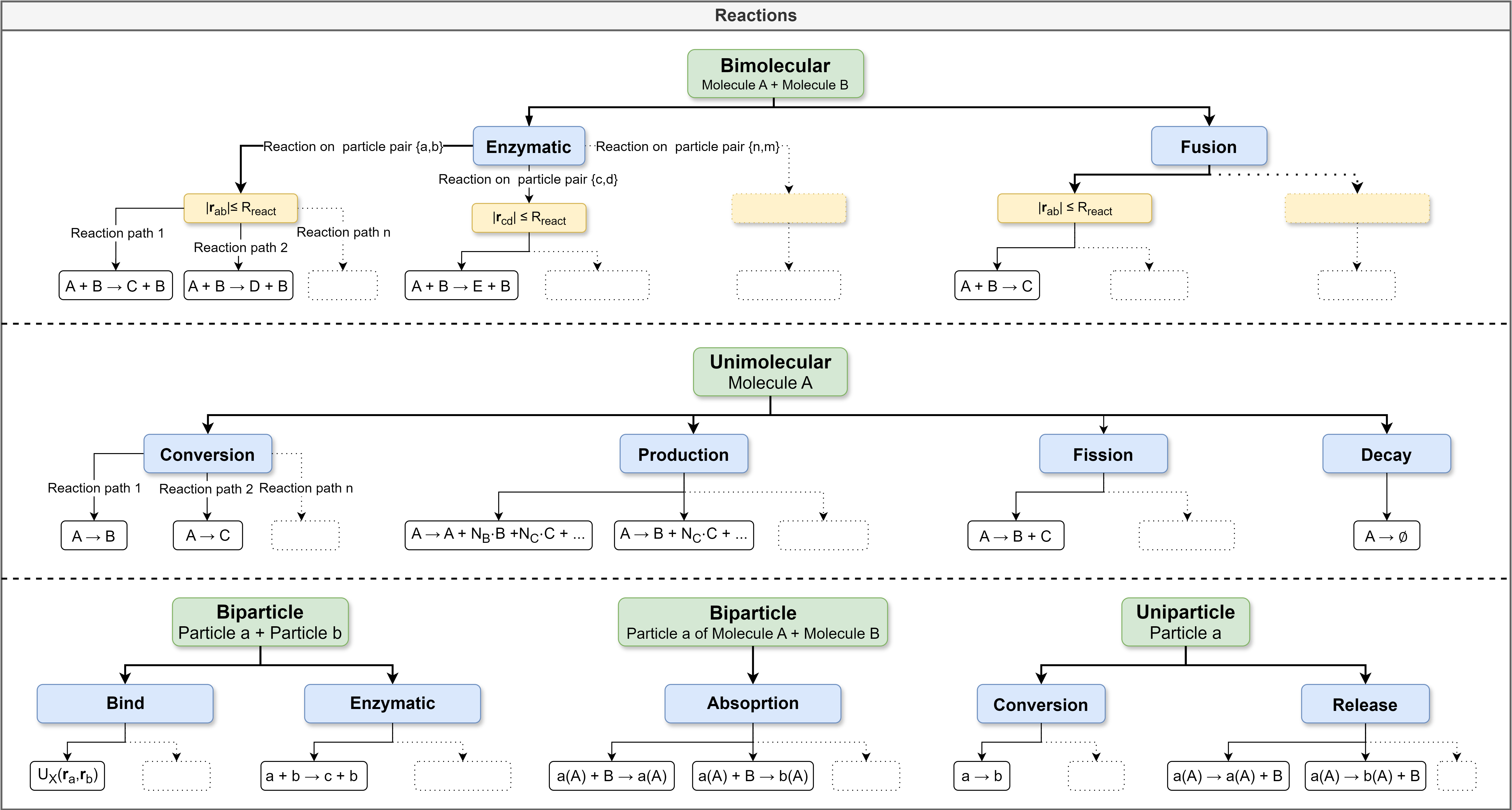
../../_images/Reactions_Graph.png — Fig. 17 **Reactions graph.** PyRID supports various kinds of bimolecular and unimolecular reactions. The trees give an overview about the possible reactions and reaction paths. Bimolecular reactions are always associated with one or several particle pairs. A reaction can always have one or several possible reaction products by having different reaction paths.

Unimolecular reactions

Unimolecular reactions include fission, conversion, and decay reactions. These can be efficiently simulated using a variant of the Gillespie Stochastic Simulation Algorithm (SSA) [12, 85]. Thereby, the time point of the next reaction is sampled from the probability distribution of expected molecule lifetimes, assuming that in between two time points no interfering event occurs. An interfering event could, e.g., be a bi-molecular reaction. The naive way of simulating uni-molecular reactions would be to check each time step whether the reaction will occur depending on its reaction rate. The Gillespie SSA has the benefit of being exact (partially true since the simulation evolves in finite, discrete time steps) and far more efficient, because we only need to evaluate a reaction once and not each time step. For a single molecule having \(n\) possible reaction paths each with a reaction rate \(k_i\), let \(k_t = \sum_i^n k_i\) be the total reaction rate. Let \(\rho(\tau) d\tau\) be the probability that the next reaction occurs within \([t+\tau,t+\tau+d\tau)\), which can be split into \(g(\tau)\), the probability that no reaction occurs within \([t,t+\tau)\) and probability that a reaction occurs within the time interval \(d\tau\), which is given by \(k_t d\tau\). Thereby,

\[\rho(\tau) d\tau = g(\tau) k_t d\tau,\]

where \(g(\tau) = e^{-k_t \tau}\) [12]. From the above equation we find \(P(\tau) = 1-e^{-k_t \tau}\) by integration. To sample from this distribution, we can use the inverse distribution function.

\[\tau = P^{-1}(U)\]

where \(U\) is uniformly distributed in \((0,1)\). From \(U = P(\tau) = 1-e^{-k_t \tau}\), we find \(P^{-1}(U) = \frac{-log(1-U)}{k_t}\). Since \(U\) is uniformly distributed in \((0,1)\), so is \(1-U\). Thereby, we can draw the time point of the next reaction from:

\[\tau = \frac{1}{k_t} \ln\Big[\frac{1}{U}\Big],\]

With the above method, we accurately sample from the distribution of expected molecule lifetimes \(\rho(\tau) = k_t e^{-k_t \tau}\).

At the time point of the reaction, we can sample from the set of reaction paths by a weighted random choice algorithm. Therefore, we compare a second random number, uniformly distributed in \((0,k_{t})\), with the cumulative set of reaction rates \((k_1, k_1+k_2, ... ,k_{t})\). The comparison can be made efficiently via a bisection algorithm.

Particle and molecule reactions

Because in PyRID, molecules are represented by rigid bead models, uni-molecular reactions can occur either on the molecule level or on the particle level. As such, if a conversion or decay reaction is defined on a molecule, executing the reaction will exchange the complete rigid bead molecule by a product molecule, or, in the case of a decay reaction, will remove the complete molecule from the simulation. On the other hand, if the reactions are defined on a particle/bead type, only the particle will be affected. Whereas decay and conversion reactions are handled very similar for molecules and particles, fission reactions are handled slightly different. Therefore, PyRID offers three types of fission reactions:

fission reactions,
production reactions,
release reactions.

Standard fission reactions can only be defined on the molecule level and are executed similar to ReaDDy [23]. Here, the number of product molecules is limited to two. In the case where educt and products are volume molecules, the product molecules are placed within a sphere of radius \(R_{fission}\). Therefore, an orientation vector \(\boldsymbol{d}\) uniformly distributed in the rotation space with a length \(<=R_{fission}\) is sampled. The two products are then placed according to

\[\begin{split}\begin{split} \boldsymbol{r}_1 = \boldsymbol{r}_0 + w_1 \boldsymbol{d}, \\ \boldsymbol{r}_2 = \boldsymbol{r}_0 - w_2 \boldsymbol{d}, \end{split}\end{split}\]

where \(\boldsymbol{r}_0\) is the center of the educt molecule. By default \(w_1 = w_2 = 0.5\). However, for different sized educts one may choose \(w_1\) and \(w_2\) proportional to the molecules diffusion coefficient or the diffusion length constant. If the educt and product molecules are surface molecules, the procedure is equivalent except that the direction vector is sampled from a disc on the mesh surface instead of from a sphere. If the educt is a surface molecule but the product a volume molecule, in addition to the sphere radius, the direction needs to be defined, .i.e whether the product is placed inside or outside the compartment. In both cases, the direction vector is not sampled from the full rotation space but only within the half-sphere cut by the triangle plane. Also, whenever a mesh compartment is present in the simulation, a ray tracing algorithm is used to resolve any collisions of the products’ direction vectors with the mesh.

production reactions: In addition to the standard fission reaction, PyRID supports reactions with more than two products, which are here called production reactions, because an educt molecule “produces” a number of product molecules. This type of reaction can, e.g., be used to simulate the influx of ions into a compartment via an ion channel. The procedure by which the reaction is executed is very similar to the fission reaction. However, here, the educt molecule is preserved but may change its type. Also, for each product molecule, a separate direction vector within a sphere of radius \(R_{prod}\) is sampled. Collisions with the mesh are handled as before, however, collisions between the product molecules are not resolved.

release reaction: PyRID also allows for a fission type reaction to be defined on particles, which is called a release reaction. Release reactions are limited to one particle and one molecule product. When a release reaction is executed, the particle is converted to the product particle type while releasing a product molecule either into the simulation volume or the surface of a mesh compartment. The latter is only possible if the rigid bead molecule the educt particle belongs to is also a surface molecule. Release reactions can, e.g., be used to simulate the release of a ligand from a specific binding site of a rigid bead molecule. The release reaction is introduced as the inverse of the particle absorption reaction (see next section on bi-molecular reactions).

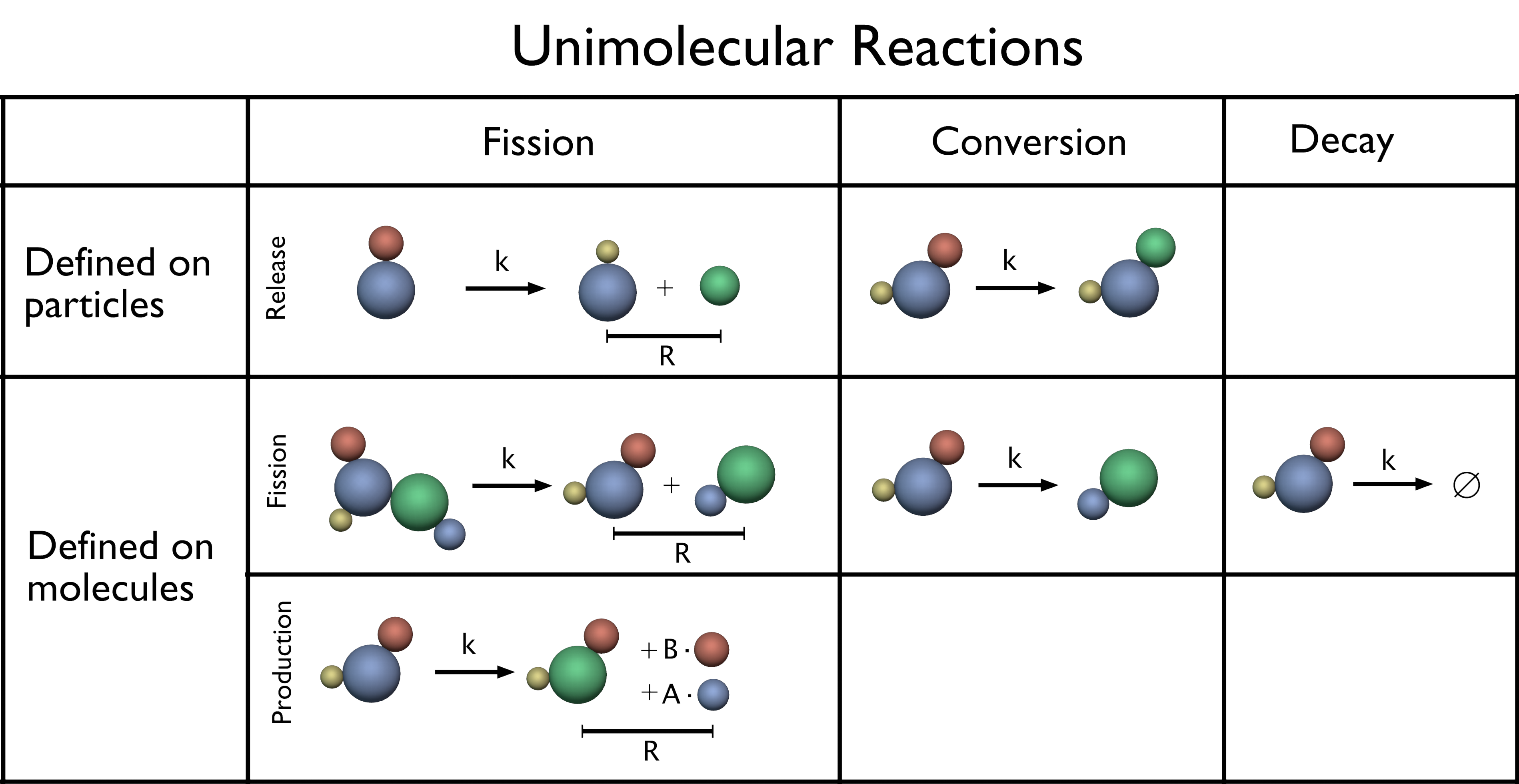
../../_images/Reactions_Overview_UM.png — Fig. 18 **Unimolecular reactions.** Unimolecular reactions can be either defined on a particle or on a molecule type. Their exist in total three different unimolecular reaction type categories: fission, conversion and decay. For details see text.

Bi-molecular reactions

Bi-molecular reactions cannot be evaluated the same way as uni-molecular reactions since we cannot sample from the corresponding probability space as we have done for the uni-molecular reactions, because we do not know when two molecules meet in advance. Here, we use a reaction scheme introduced by Doi [24], which is also used in the Brownian dynamics simulation tool ReaDDy [23, 86]. In this scheme, two molecules can only react if the inter-molecular distance \(|\boldsymbol{r}_{ij}|\) is below a reaction radius \(R_{react}\). The probability of having at least one reaction is then given by

\[p = 1-\exp\Big(-\sum_i^n k_i \Delta t \Big),\]

where \(n\) is the number of reaction paths and \(k_i\) the microscopic reaction rate for each path. Here, we distinguish between the microscopic reaction rate, which is the rate at which two molecules react if their distance is below \(R_{react}\) and the macroscopic reaction rate, which is the rate at which any two molecules react on average. The macroscopic reaction rate is what you usually get as a result out of some experimental measurement. We assume that the time step \(\Delta t\) is so small that the molecules can only undergo one reaction within \(\Delta t\). As such, the accuracy of the simulation strongly depends on the ratio between the microscopic reaction rate and the time step \(\Delta t\). If \(\sum_i^n k_i \cdot \Delta t>0.1\), PyRID will print out a warning. As for uni-molecular reactions, each bi-molecular reaction can contain several reaction paths, each of which can be of a different bi-molecular reaction type. PyRID supports the following bi-molecular reactions:

fusion reactions,
- molecule fusion,
- particle-molecule absorption,
enzymatic reactions (defined on molecules or particles),
binding reactions

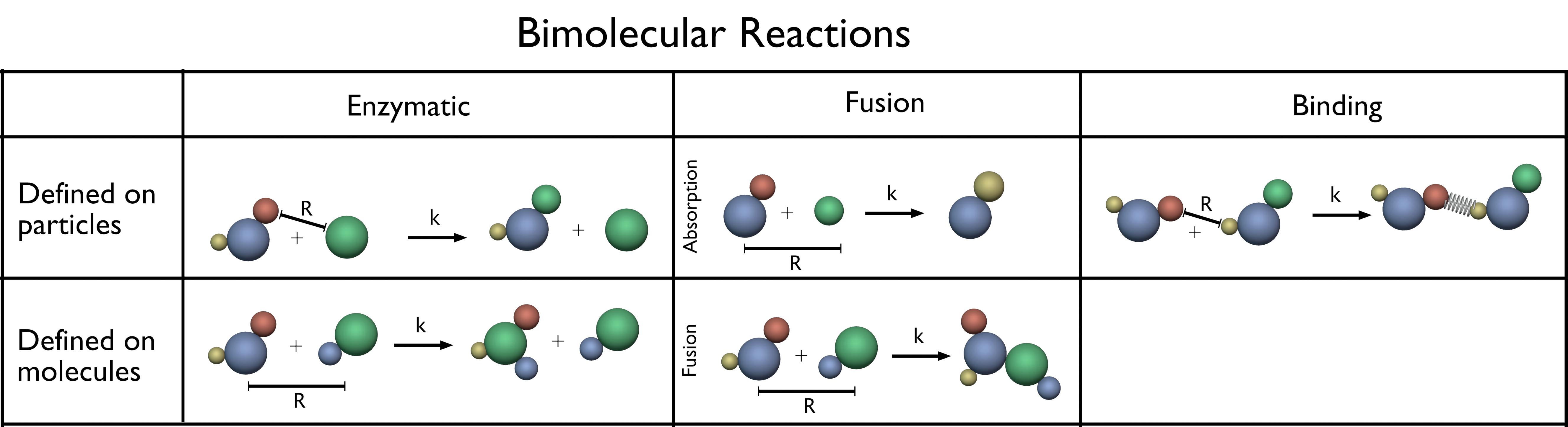
../../_images/Reactions_Overview_BM.png — Fig. 19 **Bimolecular reactions.** Bimolecular reactions can be either defined on a particle or on a molecule type. Their exist in total three different bimolecular reaction type categories: enzymatic, fusion and binding. For details see text.

Molecule fusion reactions are defined on molecule pairs. The product molecule is always placed relative to the position of the first educt. Thereby, in PyRID, the order in which the educts of a reaction are set is important. For example, for a fusion reaction \(\ce{A + B -> C}\) the product is placed at \(\boldsymbol{R}_A + \omega \Delta \boldsymbol{R}\), where \(\boldsymbol{R}_A\) is the origin of molecule \(A\), \(\Delta \boldsymbol{R}\) is the distance vector between \(A\) and \(B\) and \(\omega\) is a weight factor. For a \(\ce{B + A -> C}\), the product is placed at \(\boldsymbol{R}_B + \omega \Delta \boldsymbol{R}\). By default, \(\omega = 0.5\) such that the product is placed in the middle between the educt and the order does not matter. However, for \(\omega \neq 0.5\), the order in which the educts have been set determines where the product is placed.

In addition to the fusion reaction, PyRID offers the particle-molecule absorption reaction, which is also a reaction of the fusion type. However, here a molecule is absorbed by the bead/particle of another molecule. The molecule is thereby removed from the simulation and the absorbing particle is converted to a different type.

Binding reactions are defined between two particle/bead types and handled similar to fusion and enzymatic reactions except that, if the reaction was successful, an energy potential between the two educt particles is introduced such that these interact with each other. Upon binding, the beads can change their respective type. Also, a bead can only be bound to one partner particle at a time. Bonds can be either persistent or breakable. In the latter case, the bond is removed as soon as the inter-particle distance crosses an unbinding threshold. Similarly, unbinding reactions can be introduced by means of a conversion reaction as bonds are removed if a particle or the corresponding rigid bead molecule are converted to a different type.

Reactions between surface molecules

As for volume molecules, molecules that reside on the surface/in the membrane of a compartment react with each other if the inter-particle distance is below the reaction radius. However, PyRID only computes the euclidean distance between particles. Therefore, however, surface reactions are only accurate if the local surface curvature is large compared to the reaction radius. Accurate calculation of the geodesic distance on mesh surfaces is computationally very expensive. Algorithms that allow for relatively fast approximations of geodesic distances and shortest paths such as the Dijkstra’s algorithm often only provide good approximations for point far away from the source. Therefore, the benefit of implementing such algorithms is questionable as reaction radii are on the order of the molecule size and thereby usually small compared to the mesh size. However, much progress has been made in this field [87, 88, 89].

Potentials

PyRID supports any pairwise, short ranged interaction potential and external potentials. The force is given by

\[\boldsymbol{F}_i = \nabla_i \left( \sum U_{ext}(\boldsymbol{r}_i) + \sum_{i \neq j} U_{pair}(\boldsymbol{r}_i, \boldsymbol{r}_j) \right)\]

PyRID comes with a selection of pairwise interaction potentials. PyRID does not support methods such as Ewald summation and pair interaction potentials need to be short ranged, i.e., they need to have a cutoff distance.

In the following I list the functions currently implemented in PyRID. However, any short ranged, pair-wise interaction potential can be easily added using python.

Weak piecewise harmonic potential

The very same interaction potential is also used in ReaDDy [23].

(50)\[\begin{split}\begin{split}U_{ha}(r) = \begin{cases} \frac{1}{2}k(r-(d_1+d_2))^2-h,& \text{if } r<(d_1+d_2), \\ \frac{h}{2}(\frac{r_c-(d_1+d_2)}{2})^{-2}(r-(d_1+d_2))^2-h,& \text{if } d \le r < d + \frac{r_c-(d_1+d_2)}{2}, \\ -\frac{h}{2}(\frac{r_c-(d_1+d_2)}{2})^{-2}(r-r_c)^2,& \text{if } d + \frac{r_c-(d_1+d_2)}{2} \le r < r_c, \\ 0, & \text{otherwise} \end{cases}\end{split}\end{split}\]

Harmonic repulsion potential

The very same interaction potential is also used in ReaDDy [23].

(51)\[U(r) = \Biggl \lbrace { \frac{\kappa}{2}(r-\sigma)^2,\text{ if } { r \leq \sigma } \atop 0, \text{ otherwise }, }\]

Continuous Square-Well (CSW) potential

The Continuous Square-Well (CSW) potential has been introduced in [29].

(52)\[U_{CSW}(r) = - \frac{\epsilon_{CSW}}{2} \Big[1 - \tanh\Big(\frac{r-r_w}{\alpha}\Big)\Big].\]

Pseudo Hard Sphere (PHS) potential

The Pseudo Hard Sphere (PHS) potential has been introduced in [31].

(53)\[U_{HS} = \Biggl \lbrace { \lambda_r (\frac{\lambda_r}{\lambda_a})^{\lambda_a} \epsilon_R [(\frac{\sigma}{r})^{\lambda_r}-(\frac{\sigma}{r})^{\lambda_a}]+\epsilon_R,\text{ if } { r < (\frac{\lambda_r}{\lambda_a}) \sigma } \atop 0, \text{ if } { r < (\frac{\lambda_r}{\lambda_a}) \sigma }, }\]

Observables

PyRID can sample several different system properties:

Energy
Pressure
Virial
Virial tensor
Volume
Molecule number
Bonds
Reactions
Position
Orientation
Force
Torque
Radial distribution function

Each observable (except the volume) is sampled per molecule type or molecule/particle pair in the case of bimolecular reactions and bonds. In addition, values can be sampled in a step-wise or binned fashion. Binning is especially useful when sampling reactions as one is usually interested in the total number of reactions that occurred with a time interval and not in the number of reactions that occurred at a specific point in time. In the following I briefly describe how the radial distribution function and the pressure are calculated in PyRID.

Radial distribution function

The radial distribution function is given by

\[g(\boldsymbol{r}) = \frac{V_{box}}{N_i N_j} \left\langle \sum_{i \neq j} \delta(\boldsymbol{r}-(\boldsymbol{r}_i-\boldsymbol{r}_j)) \right\rangle = \frac{V_{box}}{N_i N_j} \frac{1}{V(\boldsymbol{r})} \sum_{i \neq j} \delta(\boldsymbol{r}-(\boldsymbol{r}_i-\boldsymbol{r}_j))\]

where \(V(\boldsymbol{r}) = \frac{4}{3} \pi (r-\Delta r)^3\) with \(\Delta r\) being the sampling bin size. \(V_{box}\) is the volume of the simulation box and \(N_i\) and \(N_j\) are the total number of molecule types \(i\) and \(j\) respectively.

Pressure

The pressure can be calculated from the virial or the the viral tensor. However, when calculating the pressure for a system of rigid bodies/ rigid bead molecules, we need to be careful how to calculate the virial tensor. Taking the inter-particle distances will result in the wrong pressure. Instead, one needs to calculate the molecular virial [35], by taking the pairwise distance between the center of diffusion of the respective molecule pairs:

\[P_{mol} = P_{mol}^{kin} + \frac{1}{6 V} \sum_{i=1}^{N} \sum_{j \neq}^{N} \langle \boldsymbol{F}_{ij} \cdot (\boldsymbol{R}_i - \boldsymbol{R}_j) \rangle,\]

where \(V\) is the total volume of the simulation box, \(\boldsymbol{F}_{ij}\) is the force on particle i exerted by particle j and \(\boldsymbol{R}_{i}, \boldsymbol{R}_{j}\) are the center of diffusion of the rigid body molecules, not the center of mass of particles i and j! In Brownian dynamics simulations, \(P_{mol}^{kin} = N_{mol} k_B T\), where \(N_{mol}\) is the number of molecules. Also, the origin of molecules is represented by the center of diffusion around which the molecule rotates about, which is not the center of mass [15]. The net frictional force and torque act through the center of diffusion. This is because when doing Brownian dynamics (and equaly for Langevin dynamics), we do account for the surrounding fluid. Different parts of the molecule will therefore interact with each other via hydrodynamic interactions/coupling. As a result, the center of the molecule (around which the molecule rotates in response to external forces) is not the same as the center of mass, which assumes no such interactions (the molecule sites in empty space). However, for symmetric molecules, the center of mass and the center of diffusion are the same.

Berendsen barostat

It is sometimes desirable to be able to do simulations in the NPT ensemble, e.g., in preparation steps to release the system from stresses. This can become necessary, e.g. when computing inter-facial properties of fluids or computing phase diagrams via direct coexistence methods [30, 32, 90]. The Berendsen barostat [91] is simple to implement and results in the correct target density of the system, however, it does not sample from the correct statistical ensemble distribution as pressure fluctuations are usually too small. By scaling the inter-particle distances, the Berendsen barostat changes the virial and thereby the system pressure. Per time step, the molecule coordinates and simulation box length are scaled by a factor \(\mu\) that is given by:

\[\mu = (1-\Delta t/\tau_P (P_0-P))^{1/3},\]

where \(\tau_P\) is the coupling time constant, \(P_0\) the target pressure. The above equation applies to an isotropic system. For a anisotropic system the equation can be generalized by substituting P with the pressure tensor. In the case of a rectangular simulation box, all tensor remain diagonal and application of the anisotropic barostat is trivial.

Distribution of molecules

Volume molecules

The distribution of molecules in the simulation volume becomes a special problem when we have mesh compartments and account for the excluded volume of the molecules. A standard approach from molecular dynamics first loosely distributes the molecules in the simulation box and then shrinks the simulation volume until a target density is reached. This approach could be transferred to a system with mesh compartments. However, here, we might also care about the compartment size. As such, we would need to choose a larger than target compartment size and shrink it until we reach the target size. If the density is too large, we may randomly delete molecules until the target density is also reached. A second approach would be to utilize the Metropolis Monte Carlo method [3] to distribute the molecules. However, this approach is more time-consuming. A third approach, which is the one we use in PyRID, uses a so-called Poisson-Disc sampling algorithm [27]. This approach has the benefit of being computationally efficient and relatively simple to implement. It, however, has the disadvantage of not reaching densities above 30% and is only well suited for approximately spherical molecules. To distribute highly aspherical molecules, currently, the only useful method that works well with PyRID is to distribute the molecules using Monte-Carlo sampling and then resolve overlaps via a soft repulsive interaction potential. If no mesh compartments are used, one may also use the Berendsen barostat at high pressure to drive the system to a high density state. The Poison-disc sampling algorithm consists of 3 steps. 1) A grid is initialized, where the cell size is set to \(r/\sqrt{3}\). 2) A sample point is created and inserted into a list of active elements. 3) While the active list is not empty, new random points around the annulus (r-2r) of the active sample points are created. If no other sample points exist within the radius r, the new sample point is accepted and inserted into the grid and the active list. If, after k trials, no new sample point is found, the active sample point is removed from the active list. For PyRID, this algorithm has been extended to account for polydisperse particle distributions.

Surface molecules

The distribution of molecules on the surface of a mesh compartment is a little more involved. Here, we utilize an algorithm introduced by Corsini et al. [25]:

Generate a sample pool S by uniformly distributing points on the mesh surface.
Divide space into cells and count the number of samples in each cell.
Randomly select a cell weighted by the number of active samples in each cell (active sample: sample that is not yet occupied or deleted).
Randomly select a sample from the selected cell.
Randomly choose a particle type of radius \(R_i\) (weighted by the relative number of each type we want to distribute).
Check whether the distance of the selected sample to the neighboring samples that are already occupied is larger or equal to Ri+Rj.
If True, accept the sample and add the molecule type and position to an occupied sample list. Next, delete all other samples within radius Ri, as these won’t ever become occupied anyway.
Update the number count of samples for the current cell.
While the desired number of molecules is not reached, return to 3. However, set a maximum number of trials.
If there are no active samples left before we reach the desired molecule number and the maximum number of trials, generate a new sample pool.

PyRID also allows the user to assign individual mesh triangles to a group and thereby define surface regions on which to distribute molecules. Example results for the distribution of volume and surface molecules using the above described methods are shown in Fig. Fig. 20.

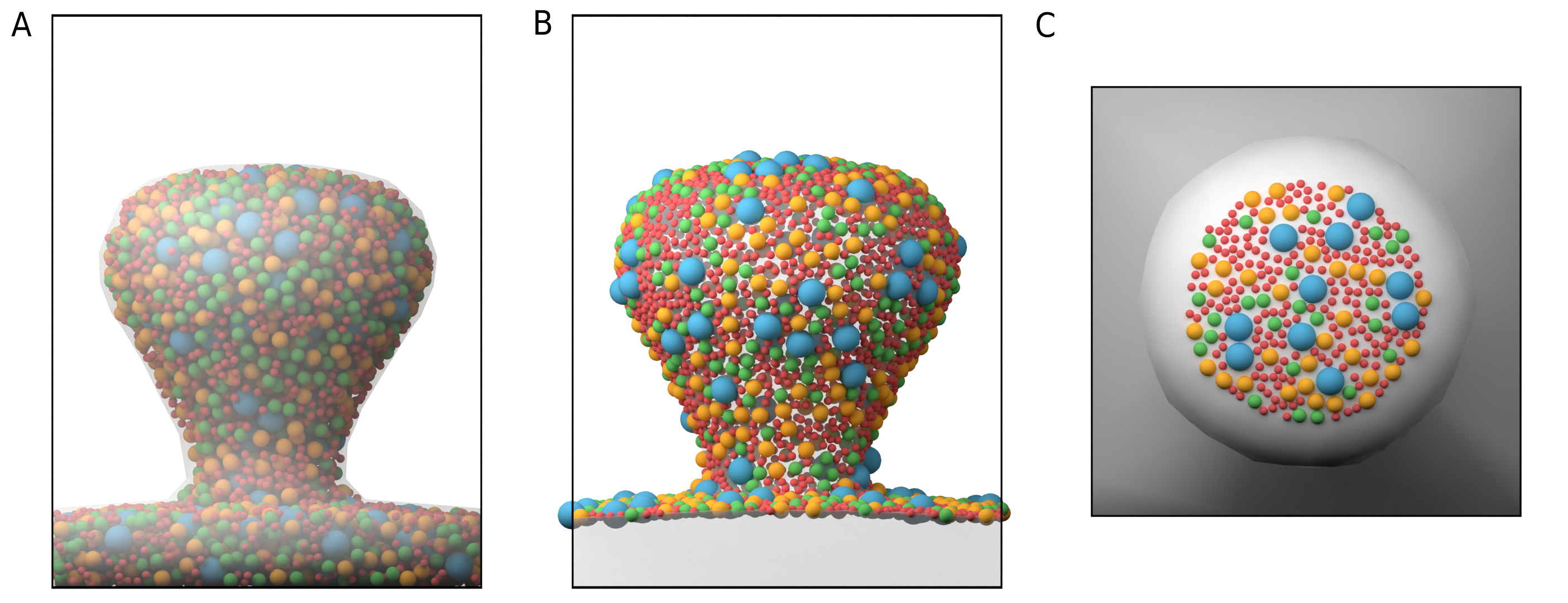
../../_images/Sphere_Packing.png — Fig. 20 **Poisson Disc Sampling of polydisperse spheres.** **(A)** Example distribution for three different sized particle types confined to the volume of a mesh compartment . **(B)** Poisson Disc sampling for surface molecules.(C) Poisson Disc sampling for surface molecules but restricted to a surface region that is defined by a triangle face group.

Fast algorithms for Brownian dynamics of reacting and interacting particles

PyRID is written entirely in the programming language python. To make the simulations run efficiently, PyRID heavily relies on jit compilation using Numba. In addition, PyRID uses a data-oriented design and specific dynamic array data structures to keep track of molecules and their reactions efficiently. For this important part of the PyRID implementation to not remain elusive, I will introduce the main data structures that make PyRID run efficiently in this section. A very nice introduction/overview to the kind of data structures used here has been written by Niklas Gray 1.

Dynamic arrays in PyRID

In PyRID, molecules and particles constantly enter or leave the system due to reactions and other events. Therefore, we need a data structure that can efficiently handle this constant change in the number of objects we need to keep track of in our simulation. The same holds true for the molecular reactions occurring at each time step. These need to be listed and evaluated efficiently. Fortunately, variants of dynamic array data structures are tailored for such tasks, of which we use two kinds, the tightly packed dynamic array and the dynamic array with holes.

The tightly packed dynamic array (dense array)

A tightly packed dynamic array is a dynamic array (similar to lists in python or vectors in C++) where elements can be quickly deleted via a pop and swap mechanism (Fig. 21). The problem with standard numpy arrays but also lists and C++ vectors is that deletion of elements is very expensive. For example, if we want to delete an element at index m of a numpy array of size n, numpy would create a new array that is one element smaller and copies all the data from the original array to the new array. Also, if we want to increase the size of a numpy array by appending an element, again, a new array will need to be created, and all data needs to be copied. This is extremely computationally expensive. One way to create a dynamic array (and python lists work in that way) is to not increase the array size each time an element is added but increase the array size by some multiplicative factor (usually 2). This consumes more memory but saves us from creating new arrays all the time. Now we simply need to keep track of the number of elements in the array (the length of the array) and the actual capacity, which can be much larger. One straightforward method to delete elements from the array is just to take the last element of the array and copy its data to wherever we want to delete an element (swapping). Next, we pop out the last element by decreasing the array length by 1. We call this type of array a ‘tightly packed array’ because it keeps the array tightly packed. One issue with this method is that elements move around. Thereby, to find an element by its original insertion index, we need to keep track of where elements move. One can easily solve this issue by keeping a second array that saves for each index the current location in the tightly packed array.

The dynamic array with holes

To store molecules and particles, we use a dynamic array with holes (Fig. 21). A dynamic array with holes is an array where elements can be quickly deleted by creating ‘holes’ in the array. These holes are tracked via a free linked list. The array with holes has the benefit over the ‘tightly packed array’ that elements keep their original index because they are not shifted/swapped at any point due to deletion of other elements. This makes accessing elements by index a bit faster compared to the other approach. However, if the number of holes is large, i.e. the array is sparse, this approach is not very cache friendly. Also, iterating over the elements in the array becomes more complex because we need to skip the holes. Therefore, we add a second array, which is a tightly packed array, that saves the indices of all the occupied slots in the array with holes (alternatively, we could add another linked list that connects all occupied slots). We can then iterate over all elements in the holes array by iterating over the tightly packed array. Keep in mind, however, that the order is not preserved in the tightly packed array, since, whenever we delete an element from the holes array, we also need to delete this element from the dense array by the pop and swap mechanism. As such, this method does not work well if we need to iterate over a sorted array. In that case, one should use a free linked list approach for iteration. As with the tightly packed dynamic array, the array size is increased by a multiplicative factor of 2 as soon as the capacity limit is reached.

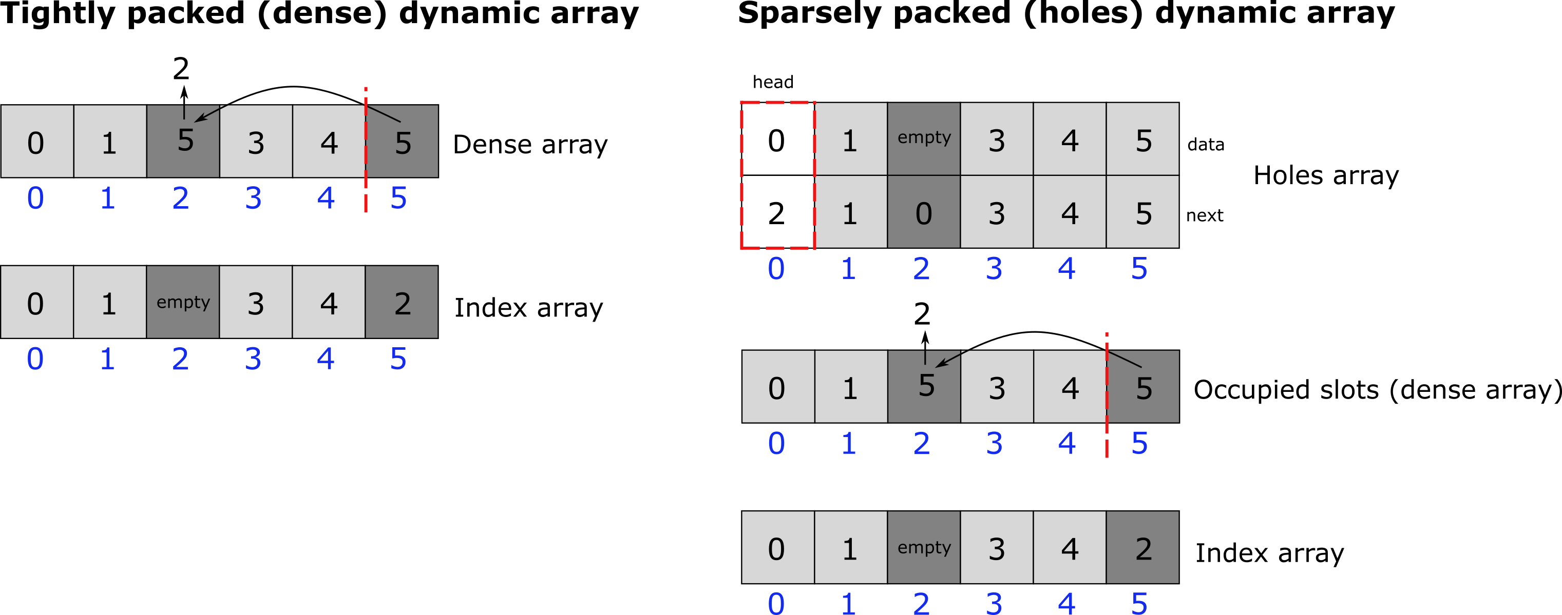
../../_images/DynamicArrays.png — Fig. 21 **Dynamic arrays.** **(A)** Tightly packed dynamic array. A tightly packed dynamic array uses a pop and swap mechanism to delete single elements. New elements are appended. Thereby, however, elements change their position. To find elements, a second, sparsely packed dynamic array is introduced that keeps track of the array index of each element. **(B)** In sparsely packed dynamic arrays, elements are deleted by creating holes. Holes are kept track of by a free linked list. Sparsely packed dynamic arrays have the benefit of keeping the position of each element inside the array fixed, which makes finding elements easy. However, this comes at the expense of more memory usage. Also, iteration over a sparse dynamic array is not straight forward as we must skip the holes in the array. Their exist different methods to iterate over such an array. In PyRID, a second, densely packed array is introduced that keeps the indices of all occupied slots. However, in order to be able to delete an element, we now also need third, sparse array, that keeps track of the element indices in the densely packed array.

Dynamic arrays used for reaction handling

The data structure we need to organize the reactions is a little bit more complex than a simple dense, dynamic array or one with holes, as is used to keep track of all the rigid body molecules and particles in the system. Instead a combination of different dynamic arrays and a hash table is used (Fig. 22). Let me motivate this: Our data structure needs to be able to do four things as efficient as possible:

Add reactions,
Delete single reactions,
Delete all reactions a certain particle participates in,
Return a random reaction from the list.

We need to be able to delete a single reaction whenever this reaction is not successful. We need to delete all reactions of a particle whenever a reaction was successful because, in this case, the particle is no longer available since it either got deleted or changed its type (except in the case where the particle participates as an enzyme). We need to be able to request a random reaction from the list because processing the reactions in the order they occur in the list would introduce a bias 2. Points 1. and 2. could be easily established with a simple dynamic array. However, point 3 is a bit more complicated but can be solved with a doubly free linked list embedded into a dynamic array with holes. This doubly linked list connects all reactions of a particle. To find the starting point (the head) of a linked list within the array for a certain particle, we save the head in a hash table (python dictionary). A doubly linked list is necessary because we need to be able to delete a single reaction (of index k) from the linked list (point 2). As such, we need to be able to reconnect the linked list’s ‘chain’. Therefore, we need to know the element in the linked list that pointed to k (previous element) in addition to the element/reaction k points to (next element). Another problem that needs to be solved is that a reaction can be linked to at maximum two educts. Therefore, each next and previous pointer needs to be 4-dimensional: We need one integer for each educt to save the next (previous) reaction index and another integer 0,1 to keep track of whether in the next (previous) reaction, the particle is the first or the second educt, because this may change from reaction to reaction! Since the dynamic array, the doubly linked list is embedded, in has holes, picking a random reaction from the list becomes another issue. This can, however, easily be solved by adding another dynamic array (tightly packed), which keeps the indices of all the reactions that are left in a tightly packed format. Picking a random reaction is then as easy as drawing a uniformly distributed random integer between 0 and n, where n is the length of the dense array.

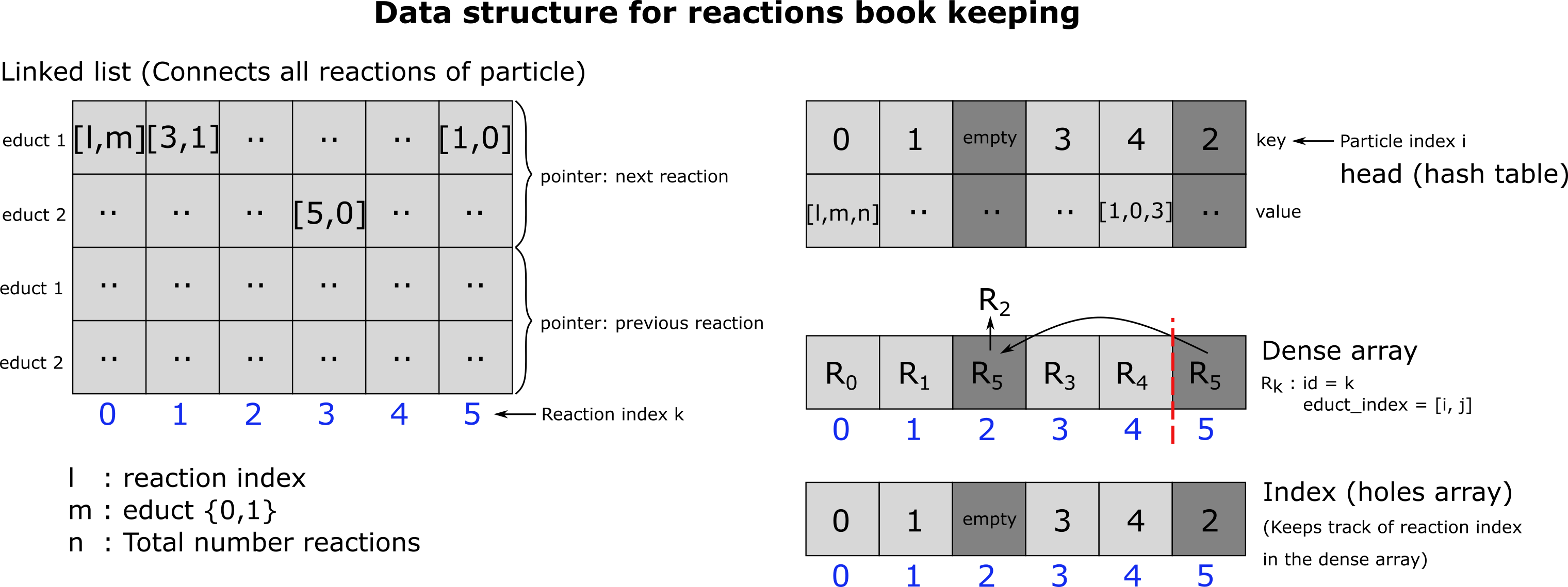
../../_images/Reactions_DynamicArray1.png — Fig. 22 **Dynamic array for reactions.** The dynamic array that keeps track of all the reactions that need to be executed within a simulation time step consists a free doubly linked list, a hash table (python dictionary), one densely packed and one sparsely packed dynamic array.

Polydispersity

A problem that needs to be addresses, especially when using minimal coarse-graining approaches with low granularity is polydispersity of particle radii. One extreme example would, e.g., be a simulation where proteins and synaptic vesicles are represented by single particles. In this case classical linked cell list algorithms become highly inefficient.

The computationally most expensive part in molecular dynamics simulations is usually the calculation of the pairwise interaction forces, because to calculate these, we need to determine the distance between particles. When doing this in the most naive way, i.e. for each particle i we iterate over all the other particles j in the system and calculate the distance, the computation time will increase quadratic with the number of particles in the system (\(O(N^2)\)). Even if we take into account Newtons third law, this will decrease the number of computations (\(O(\frac{1}{2}N(N-1))\)), but the computational complexity still is quadratic in N. A straight forward method to significantly improve the situation is the linked cell list approach [3] (pp.195: 5.3.2 Cell structures and linked lists) where the simulation box is divided into \(n \times n \times n\) cells. The number of cells must be chosen such that the side length of the cells in each dimension \(s = L/n\), where \(L\) is the simulation box length, is greater than the maximum cutoff radius for the pairwise molecular interactions (and in our case also the bimolecular reaction radii). This will decrease the computational complexity to \(O(14 N \rho s^3 )\), where \(\rho\) is the molecule density (assuming a mostly homogeneous distribution of molecules). Thereby, the computation time increase rather linear with \(N\) instead of quadratic (\(N^2\)).

However, one problem with this method is that it does not efficiently handle polydisperse particle size distributions. This becomes a problem when doing minimal coarse graining of proteins and other structures we find in the cell such as vesicles. As mentioned above, n should be chosen such that the cell length is greater than the maximum cutoff radius. If we would like to simulate, e.g. proteins (\(r \approx 2-5 nm\)) in the presence of synaptic vesicles (\(r \approx 20-30 nm\)), the cells become way larger than necessary from the perspective of the small proteins.

One way to approach this problem would be, to choose a small cell size (e.g. based on the smallest cutoff radius) and just iterate not just over the nearest neighbour cells but over as many cells such that the cutoff radius of the larger proteins is covered. This approach has a big disadvantages: Whereas for the smaller particles we actually reduce the number of unnecessary distance calculations, we do not for the larger particles as we iterate over all particles, also those, which are far beyond the actual interaction radius. We can, however, still take advantage of Newton’s 3rd law. For this, we only do the distance calculation if the radius of particle i is larger than the radius of particle j. If the radii are equal, we only do the calculation if index i is smaller than index j.

A much better approach has been introduced by Ogarko and Luding [4] that makes use of a so called hierarchical grid. This approach is the one I use in PyRID. In the hierarchical grid approach, each particle is assigned to a different cell grid depending on its cutoff radius, i.e. the grid consists of different levels or hierarchies, each having a different cell size. This has the downside of taking up more memory, however, it drastically reduces the number of distance calculations we need to do for the larger particles and also takes advantage of Newtons third law, enabling polydisperse system simulations with almost no performance loss. The algorithm for the distance checks works as follows [4]:

Iterate over all particles
Assign each particle to a cell on their respective level in the hierarchical grid
Iterate over all particles once more
Do a distance check for the nearest neighbour cells on the level the current particle sites in. This is done using the classical linked cell list algorithm.
Afterwards, do a cross-level search. For this, distance checks are only done on lower hierarchy levels, i.e. on levels with smaller particle sizes than the current one. This way, we do not need to double check the same particle pair (Newtons 3rd law). However, in this step, we will have to iterate over potentially many empty cells.

Simulation loop

At the beginning of each iteration, PyRID updates the position of all particles. Next, PyRID determines the particle pair distances and based on that calculates the forces and adds reactions to the reactions list. Then, the reactions are performed. Thereby, new particles can enter the system, either by a fusion or a fission reactions. In principle, the inter-particle distances as well as the forces would need to be updated. However, to save computation time this step is skipped. The only exceptions are binding reactions, for which the force is calculated at the time of reaction execution. Thereby, in the beginning of the next iteration, the reaction products diffuse freely as they did not experience any forces yet and the trajectory of particles that have been in the system before also is not altered due to the presence of the new molecules. Also, for molecules that where converted to a different type the forces that are taken into account for the upcoming position update are those that the molecule experienced before the type change. This is of course an approximation but saves us from updating the particle distances twice. For small integration time steps the error introduced by this scheme should be small. Also, the product molecule placement itself does already not resolve any collisions and other interactions with nearby molecules. Therefore, a very similar error is introduced anyway since resolving collisions would be unfeasible and take up too much computation time. For fission reactions the error will be very similar, no matter whether forces are updated or not. For fusion reactions the the situation is slightly different because the educts will leave behind an empty space that will be filled with new molecules. But, also here, the error should be small for small time steps, which need to be considered anyhow as soon as interactions are introduced. A problem will always arise as soon as the system is dense and many products enter the system at ones. In this case, the integration time step should be decreased such that only a few products enter the system.

An alternative to the above approach would be to calculate all the forces and add all the reactions to the reactions list at the beginning of each iteration. Next we would update the molecule positions and only then evaluate the reactions. This approach has the benefit that for the product molecules, the forces will be evaluated directly after they have been placed. However, because the products are only placed after the molecule positions are updated, this results in a bias, especially for bimolecular reactions. The first approach has the benefit that it does not introduce any bias in the case where we do not consider interactions. Therefore, this is the approach I took with PyRID. In contrast, ReaDDy does update the neighbouring list for the molecules twice per iteration. Once to evaluate the reactions and another time to update the forces. However, in the worst case this could increase computation time by a factor of two if the update of inter-molecular distances is not optimized in some way. With the approach I took, forces and reactions are evaluated in one loop over all particle pairs in the neighbouring list and pair distances are calculated only once. One could try to optimize the update of pair distances after the reactions have been executed, since the pair distances between most particles stays the same and we only need to consider those particles that left or entered the system. However, this will be future work.

Visualization

For visualization, I have developed a blender addon for PyRID. In addition, PyRID can visualize the different reactions using graphs. Graph visualization in PyRID is build upon the pyvis library.

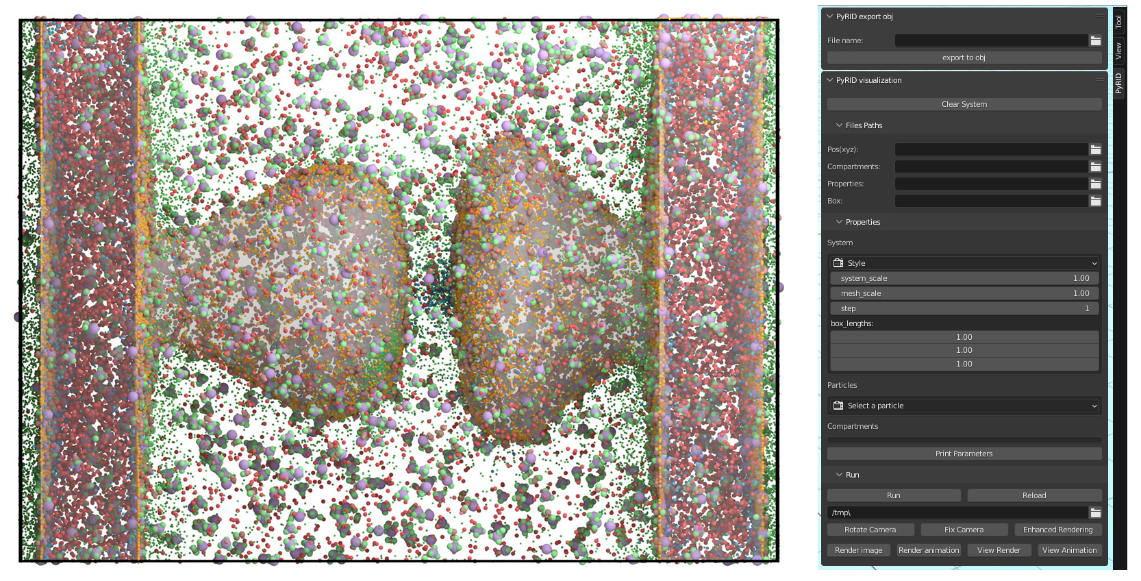
../../_images/blender_addon.jpg — Fig. 23 **Visualization of molecule trajectories with PyRIDs Blender addon.** Left: Example visualization with 50.000 particles. Right: GUI of the Blender addon.

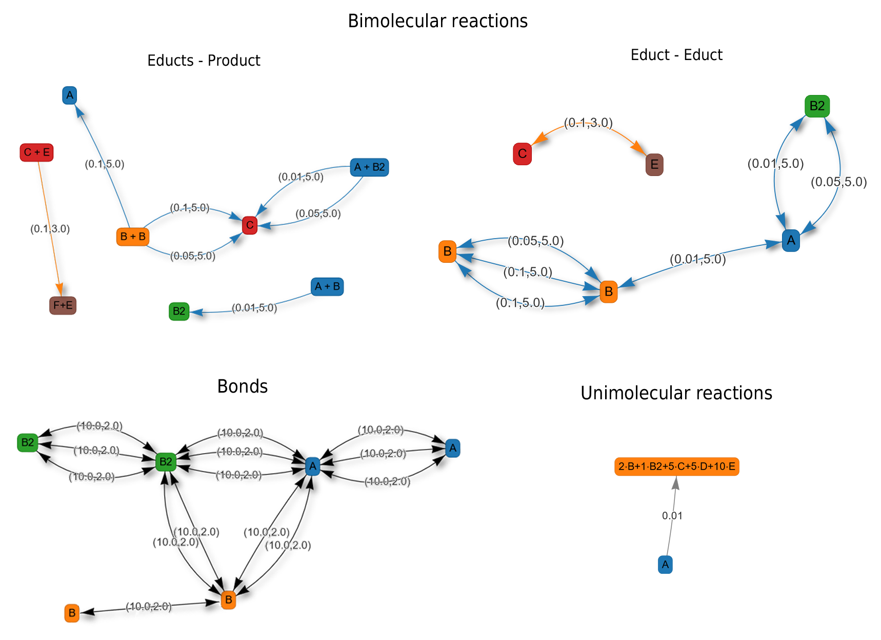
../../_images/ReactionsGraphs_Vis.png — Fig. 24 **Examples of different reaction graphs.**

1: https://web.archive.org/web/20220517145529/https://ourmachinery.com/post/data-structures-part-1-bulk-data/ https://web.archive.org/web/20220314011542/https://ourmachinery.com/post/data-structures-part-2-indices/ https://web.archive.org/web/20220517134710/https://ourmachinery.com/post/data-structures-part-3-arrays-of-arrays/ https://www.gamedeveloper.com/programming/data-structures-part-1-bulk-data
2: Reactions of particles with a low index are added to the reaction list first, because particle distances are evaluated in the order particles occur in the corresponding list (which is, at least in the beginning, in ascending order, when the indices of particles have not yet been swapped around a lot). Thereby particle one would always have a higher chance of having a successful reaction when competing with other particles.